BigBite Optics #8
Matrix elements "[TgPh|FpPh]" and "[TgTh|x]"
Matlab Calibration & new Matrix:
Last week I mentioned that I am working on the optics calibration algorithm in Matlab.
The code seems to be working now. So far I have been able to find matrix elements
for variables "TgPh" and "TgTh". In this iteration I have considered matrix elements up
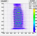
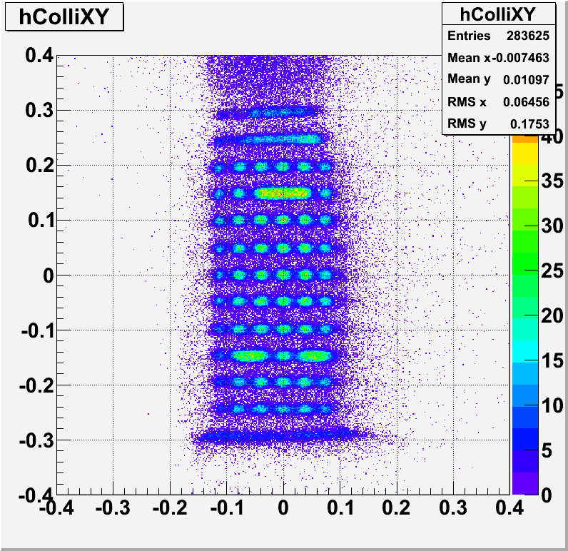
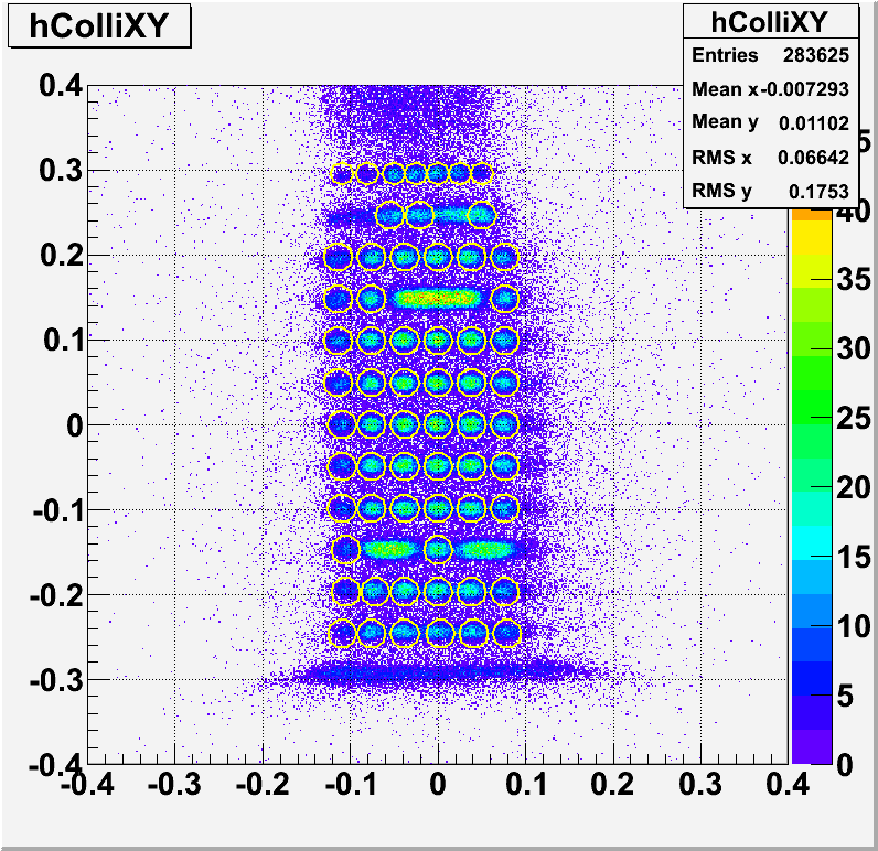
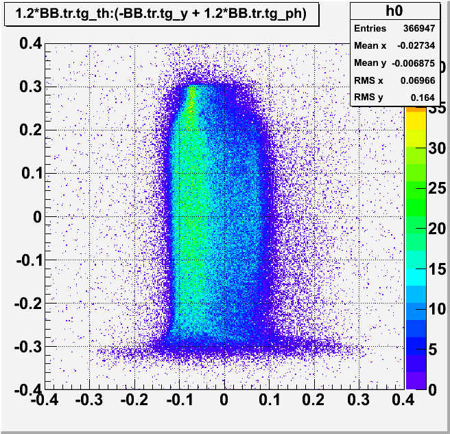
to the forth order. Here are the results. With this new procedure the sieve pattern got
a bit better. Now we can see most-left holes of the sieve. We can also see additional
series of holes in the bottom (line of holes before last), that were not visible before. However,
this matrix still does not transform correclty events from the most upper portion of the
sieve. At the moment we are trying to solve this problem. We believe that to describe this
behaviour we need even higher order matrix elements (fifth order ?) However, we believe that
we alredy have to many matrix elements (70) and consistent introducion of fifth order elements would mean
additional 60 terms. This will not do. Therefore we will first try to reduce number of the
existing matix elements by neglecting the unimportant matrix elements and than intoduce
some new matrix elements by hand, to describe behaviour on the top of the sieve.
Hopefully this will work.
1.) 
[matrix]
t 1 0 0  0.0000E+00  0.0000E+00  0.0000E+00  0.0000E+00  0.0000E+00  0.0000E+00   0.0000E+00
y 1 0 0  0.0000E+00  0.0000E+00  0.0000E+00  0.0000E+00  0.0000E+00  0.0000E+00   0.0000E+00
p 1 0 0  0.0000E+00  0.0000E+00  0.0000E+00  0.0000E+00  0.0000E+00  0.0000E+00   0.0000E+00

D 0 0 0  -0.0062343  -0.9545440  1.13910000  0.0000E+00  0.0000E+00  0.0000E+00   0.0000E+00
D 1 0 0  3.39098000  -7.6819500  7.76604000  0.0000E+00  0.0000E+00  0.0000E+00   0.0000E+00
D 2 0 0  11.7304000  -19.230500  21.1691000  0.0000E+00  0.0000E+00  0.0000E+00   0.0000E+00
D 3 0 0  14.3041000  -8.6769400  3.53875000  0.0000E+00  0.0000E+00  0.0000E+00   0.0000E+00

T 0 0 0  -0.013657   -0.51363    0.058716    0.059744   -0.059852
T 1 0 0   0.45305     0.023602  -0.15936     0.084532    0.0
T 2 0 0  -0.016576    0.12177   -0.016977    0.0         0.0
T 3 0 0  -0.018396   -0.065876   0.0         0.0         0.0
T 4 0 0   0.063481    0.0        0.0         0.0         0.0
T 0 1 0   0.0018086   0.027319   0.021888    0.067522    0.0
T 0 2 0  -0.038123    0.023323   0.53049     0           0.0
T 0 3 0   0.045988   -0.10698    0.0         0           0
T 0 4 0  -0.064298    0          0           0           0
T 0 0 1  -0.0074584  -0.093952  -0.016637   -0.027579    0.0
T 0 0 2   0.14881     0.30279   -0.64125     0.0         0.0
T 0 0 3  -0.18883     2.727      0.0         0.0         0.0
T 0 0 4  -0.15256     0.0        0.0         0.0         0.0
T 0 1 1  -0.10201    -0.40498   -0.028072    0.0         0.0
T 0 2 1   0.11611    -0.52558    0.0         0.0         0.0
T 0 3 1  -1.0489      0.0        0.0         0.0         0.0
T 0 1 2   0.0081171  -0.49757    0.0         0.0         0.0
T 0 2 2   1.3538      0.0        0.0         0.0         0.0
T 0 1 3  -0.078287    0.0        0.0         0.0         0.0
T 1 0 1   0.062559    0.19332    0.089416    0.0         0.0
T 2 0 1  -0.18283     0.33515    0.0         0.0         0.0
T 3 0 1  -0.25355     0.0        0.0         0.0         0.0
T 1 0 2  -0.53321     0.18428    0.0         0.0         0.0
T 2 0 2   0.67786     0.0        0.0         0.0         0.0
T 1 0 3  -2.7152      0.0        0.0         0.0         0.0
T 1 1 0  -0.0092399  -0.12064    0.052921    0.0         0.0
T 2 1 0   0.13073    -0.62477    0.0         0.0         0.0
T 3 1 0   0.46124     0.0        0.0         0.0         0.0
T 1 2 0  -0.013574   -0.73554    0.0         0.0         0.0
T 2 2 0   0.54637     0.0        0.0         0.0         0.0
T 1 3 0  -1.4077      0.0        0.0         0.0         0.0
T 1 1 1   0.81748    -0.075751   0.0         0.0         0.0
T 1 1 2  -2.1847      0.0        0.0         0.0         0.0
T 2 1 1   0.097293    0.0        0.0         0.0         0.0
T 1 2 1   5.1688      0.0        0.0         0.0         0.0

P 0 0 0  -0.0088043   0.0096823  0.018803   -0.040228   -0.036426
P 1 0 0  -0.0042762  -0.049541   0.066498    0.12828     0.0
P 2 0 0   0.045487   -0.01505   -0.1612      0.0         0.0
P 3 0 0  -0.016359    0.18229    0.0         0.0         0.0
P 4 0 0  -0.13618     0.0        0.0         0.0         0.0
P 0 1 0  -0.032741    0.031824   0.20345    -0.88558     0.0
P 0 2 0  -0.07643     0.41547   -1.1894      0.0         0.0
P 0 3 0   0.43283     0.102      0.0         0.0         0.0
P 0 4 0  -0.021538    0.0        0.0         0.0         0.0
P 0 0 1   1.015      -0.20526   -0.081301    0.45262     0.0
P 0 0 2   0.24439     0.61772   -0.27485     0.0         0.0
P 0 0 3   0.11516    -0.11862    0.0         0.0         0.0
P 0 0 4  -0.95747     0.0        0.0         0.0         0.0
P 0 1 1   0.11332    -0.89997    0.47398     0.0         0.0
P 0 2 1   0.36089     0.098777   0.0         0.0         0.0
P 0 3 1  -0.72964     0.0        0.0         0.0         0.0
P 0 1 2  -1.1341      0.90106    0.0         0.0         0.0
P 0 2 2  -0.40789     0.0        0.0         0.0         0.0
P 0 1 3  -2.4801      0.0        0.0         0.0         0.0
P 1 0 1  -0.057121    0.015668   0.71129     0.0         0.0
P 2 0 1  -0.35644    -1.358      0.0         0.0         0.0
P 3 0 1  -0.32484     0.0        0.0         0.0         0.0
P 1 0 2   0.16946     0.54635    0.0         0.0         0.0
P 2 0 2  -1.4447      0.0        0.0         0.0         0.0
P 1 0 3  -1.133       0.0        0.0         0.0         0.0
P 1 1 0   0.1277     -0.50393    0.96598     0.0         0.0
P 2 1 0   0.71264     0.12188    0.0         0.0         0.0
P 3 1 0   0.35199     0.0        0.0         0.0         0.0
P 1 2 0  -0.3668      2.9476     0.0         0.0         0.0
P 2 2 0  -1.3738      0.0        0.0         0.0         0.0
P 1 3 0   0.086291    0.0        0.0         0.0         0.0
P 1 1 1   0.26917    -1.1322     0.0         0.0         0.0
P 1 1 2   0.13742     0.0        0.0         0.0         0.0
P 2 1 1   0.01714     0.0        0.0         0.0         0.0
P 1 2 1   0.44885     0.0        0.0         0.0         0.0


Y 0 0 0  -0.0321556  0.0000E+00  0.0000E+00  0.0000E+00  0.0000E+00  0.0000E+00   0.0000E+00
Y 0 1 0  -1.0241000  0.0000E+00  0.0000E+00  0.0000E+00  0.0000E+00  0.0000E+00   0.0000E+00
Y 0 2 0  -0.4919260  0.0000E+00  0.0000E+00  0.0000E+00  0.0000E+00  0.0000E+00   0.0000E+00
Y 0 0 1  2.8077500  0.0000E+00  0.0000E+00  0.0000E+00  0.0000E+00  0.0000E+00   0.0000E+00
Y 0 1 1  0.72023300  0.0000E+00  0.0000E+00  0.0000E+00  0.0000E+00  0.0000E+00   0.0000E+00
Y 0 2 1  -0.7153320  0.0000E+00  0.0000E+00  0.0000E+00  0.0000E+00  0.0000E+00   0.0000E+00
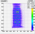
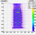
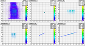
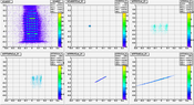
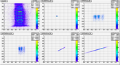
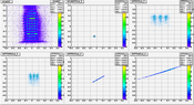
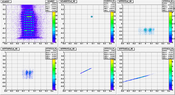
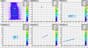
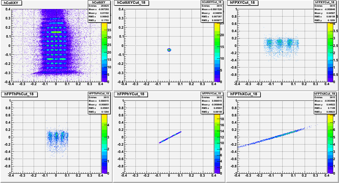
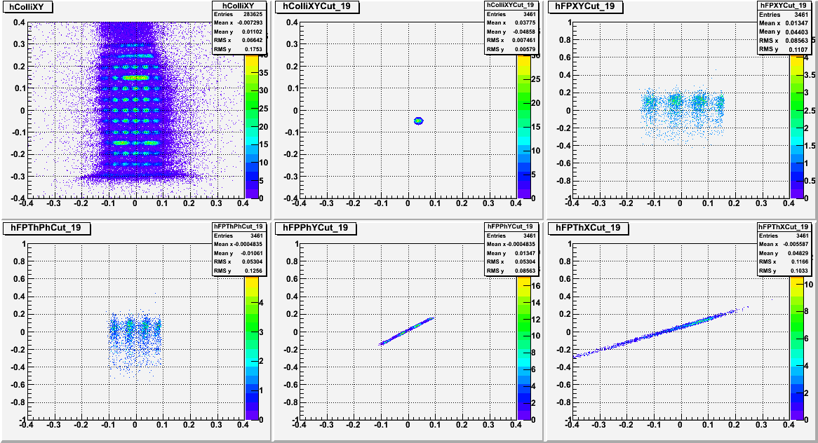
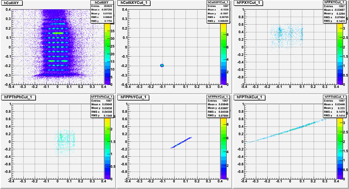
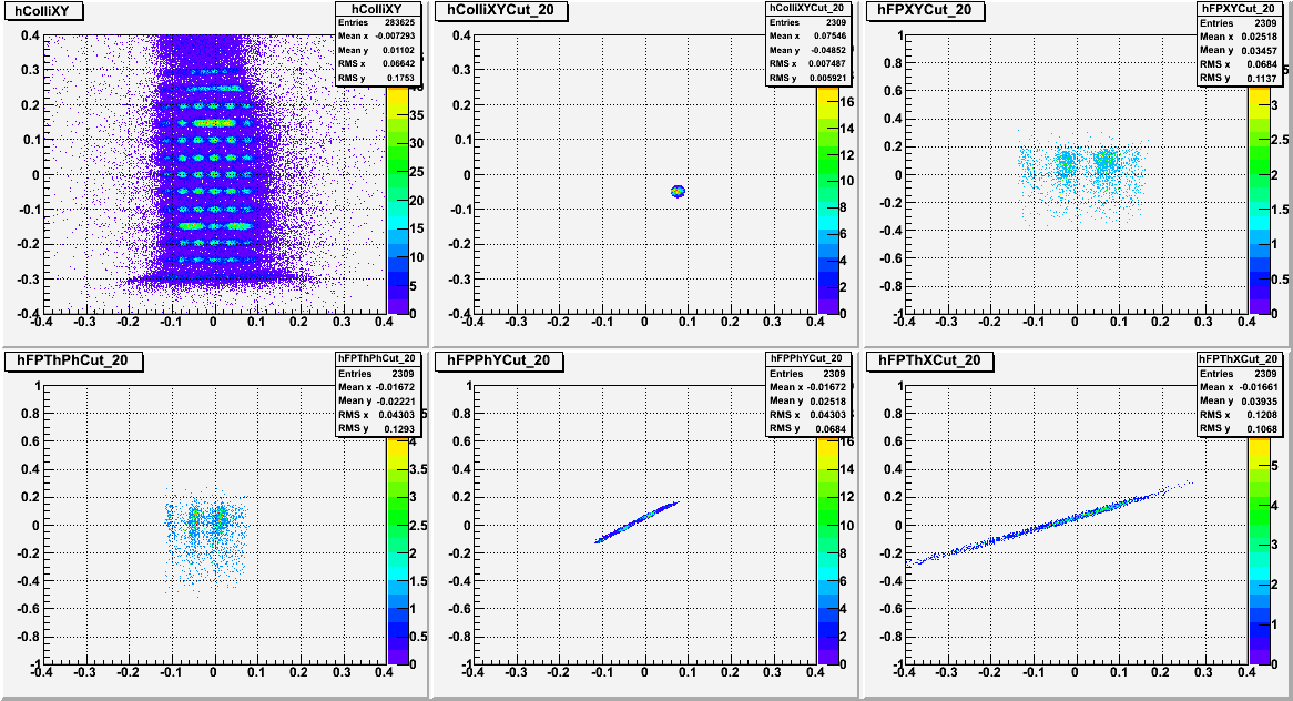
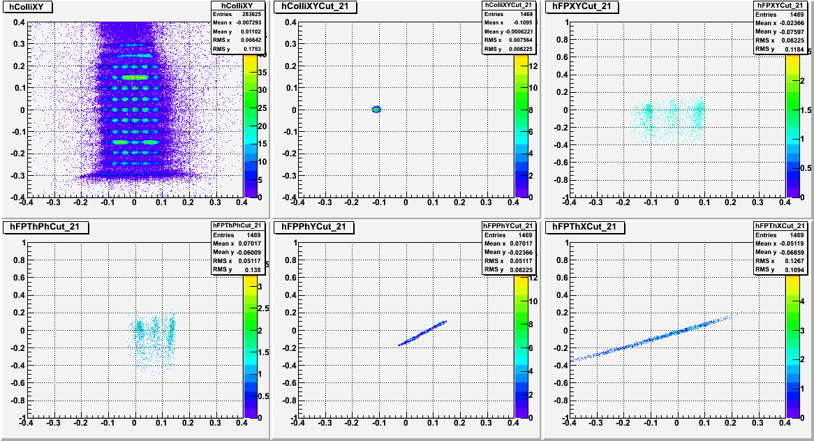
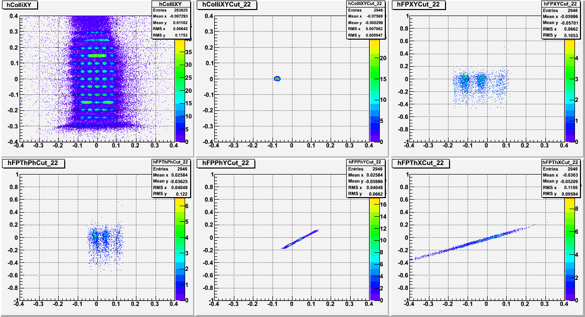
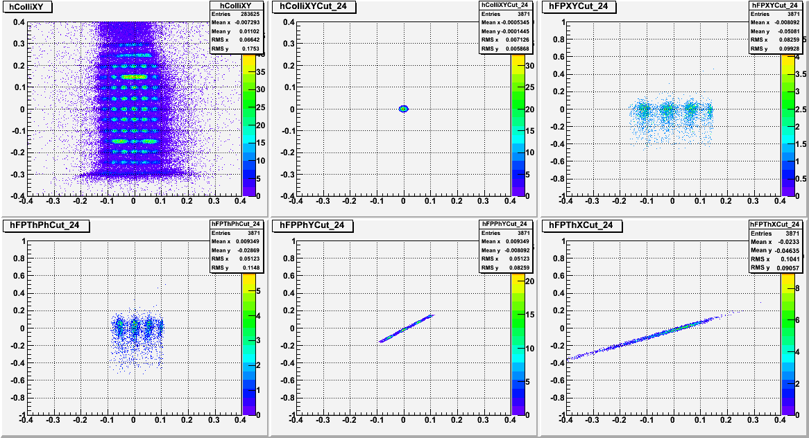
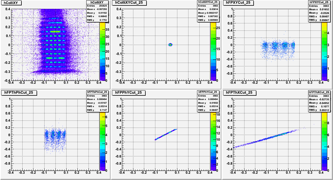
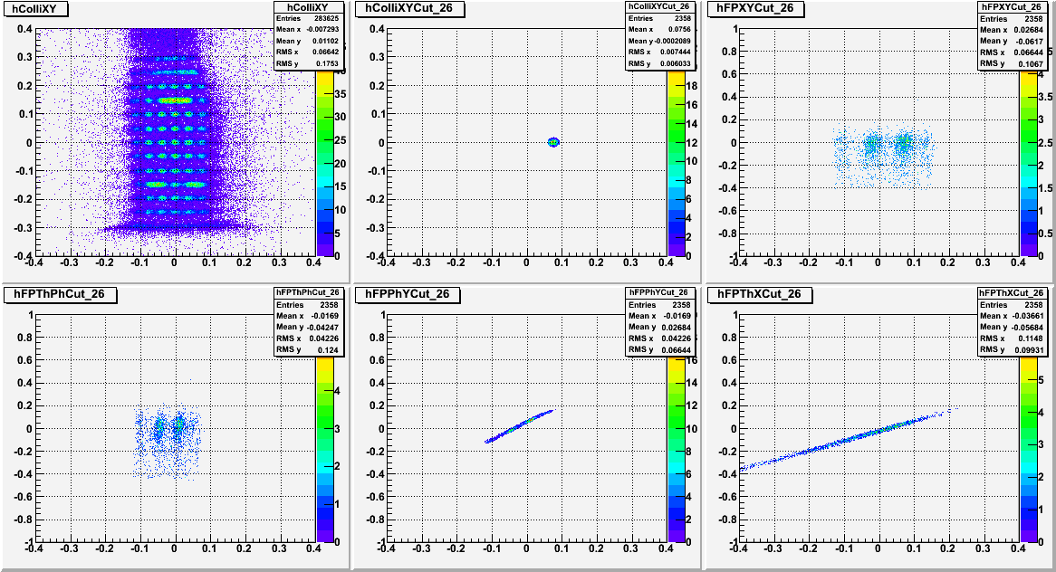
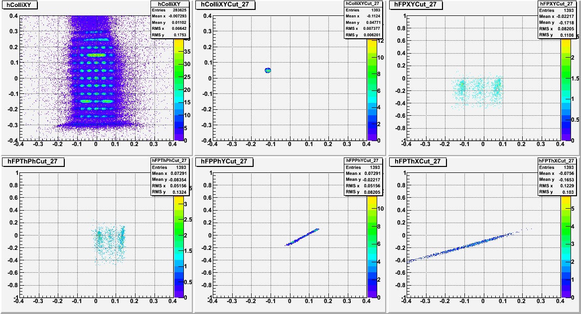
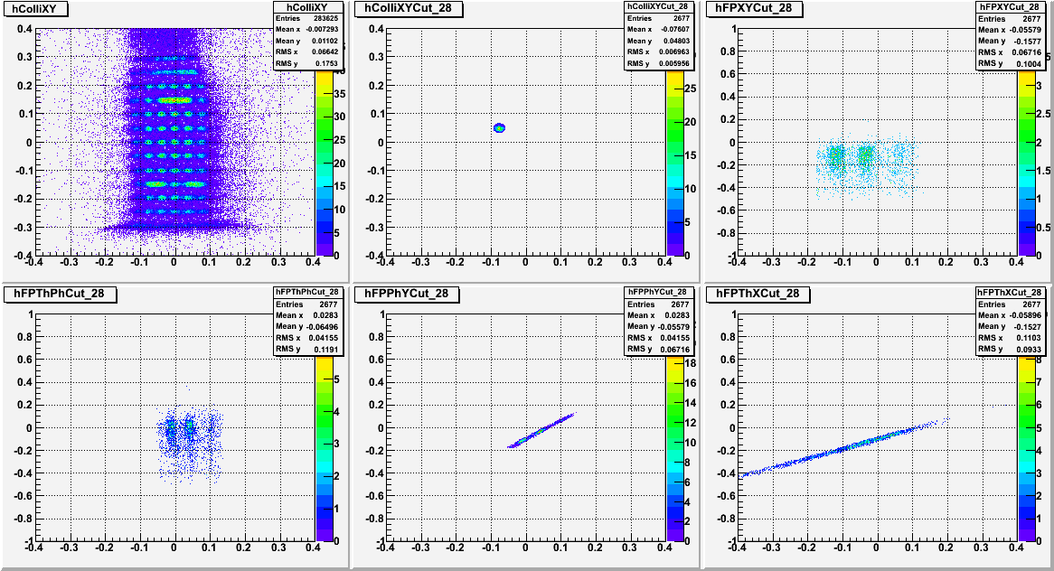
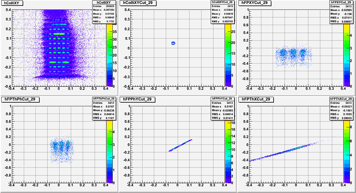
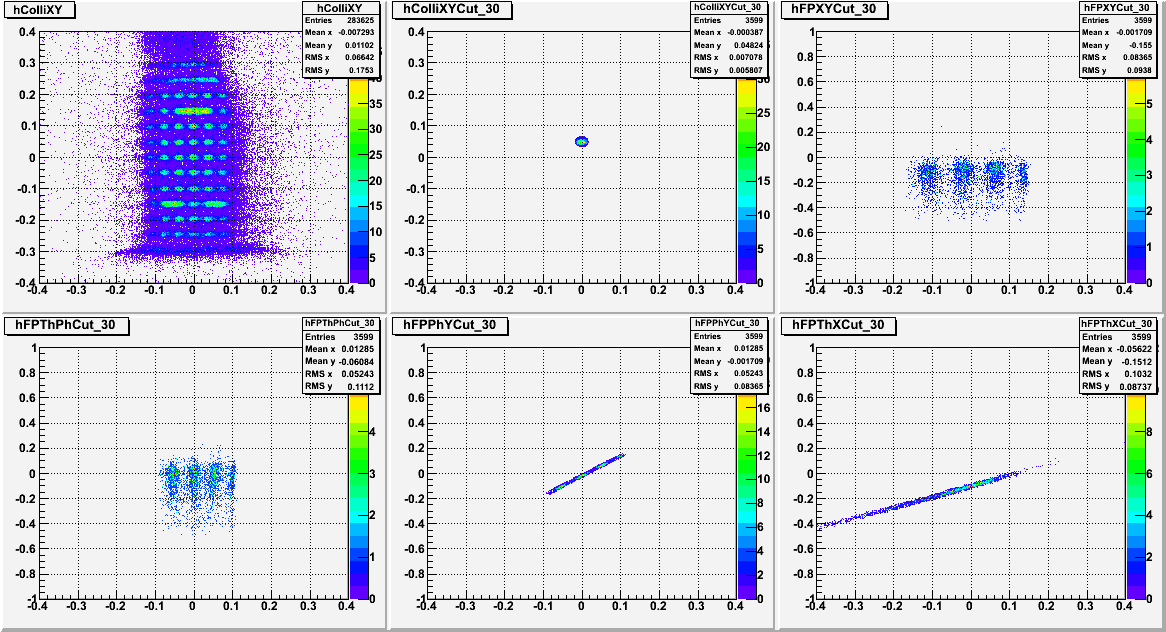
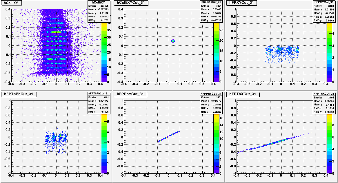
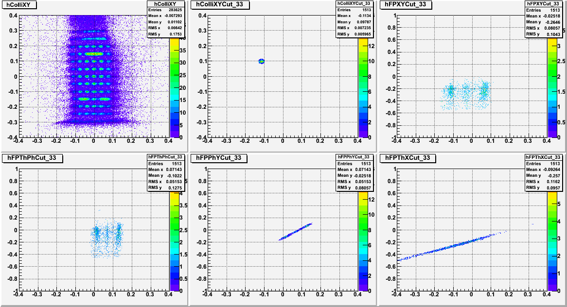
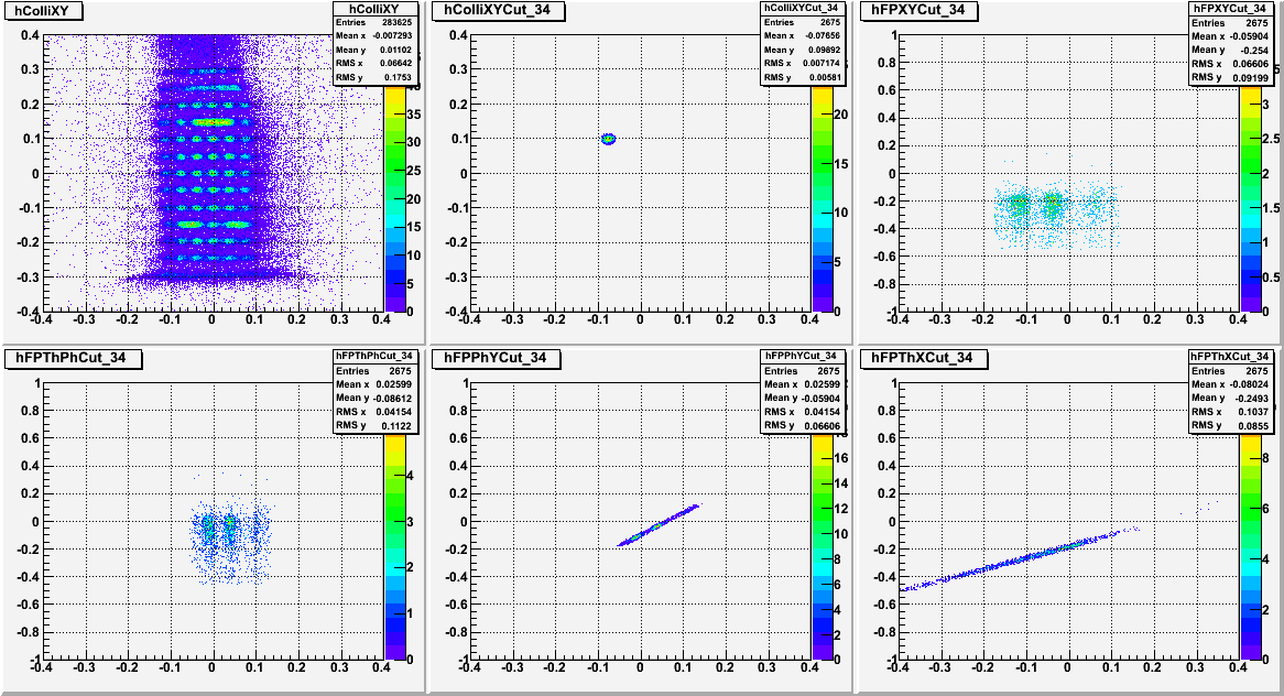
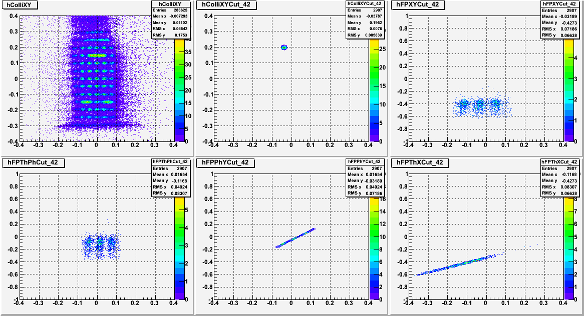
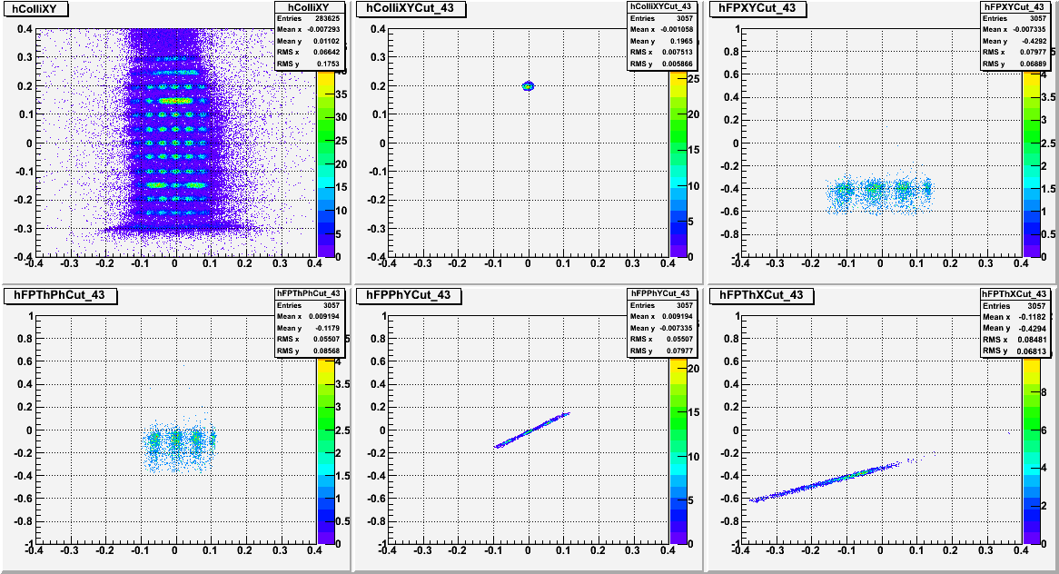
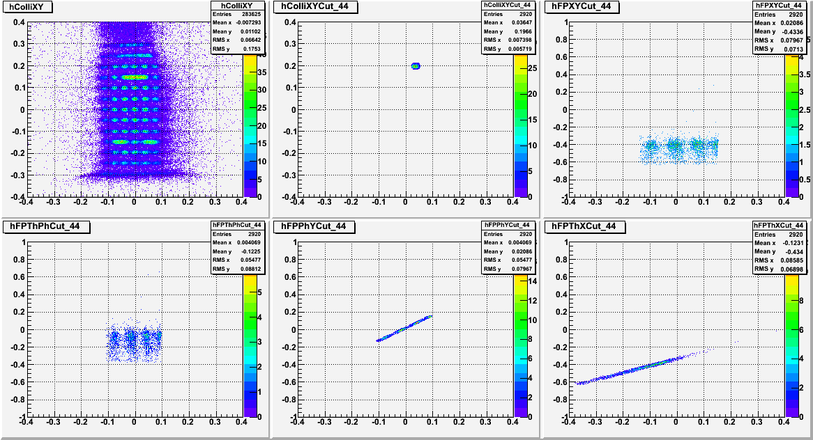
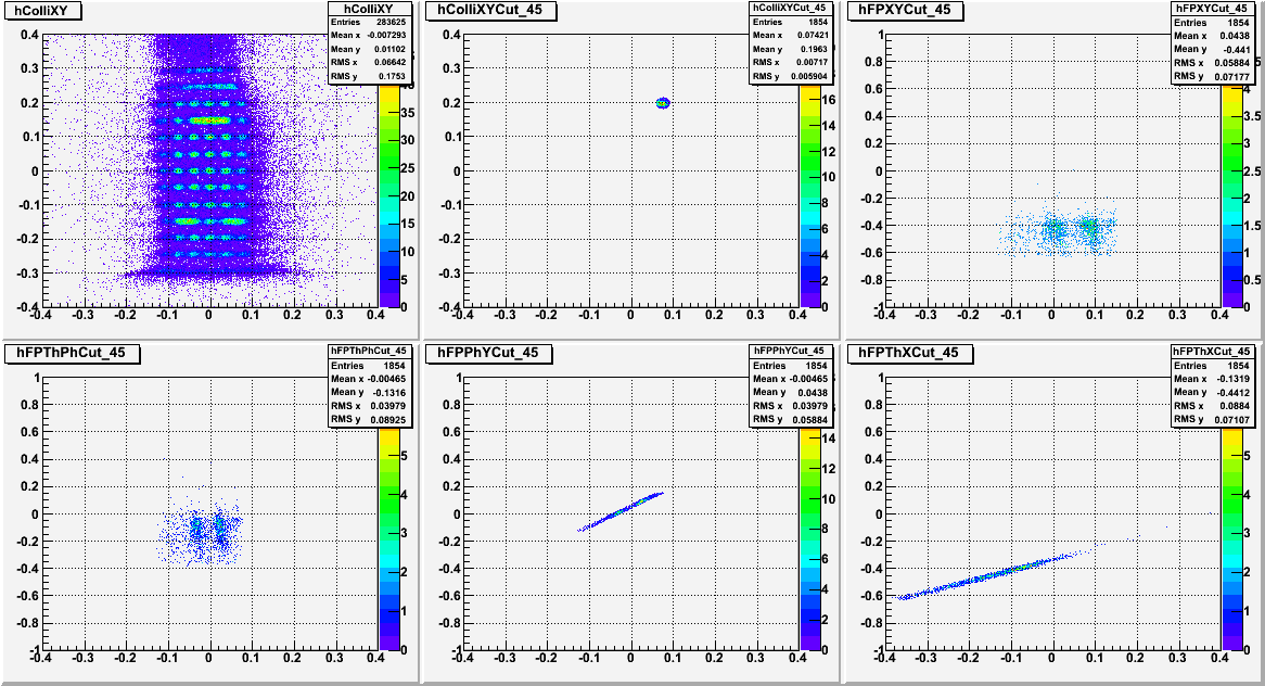
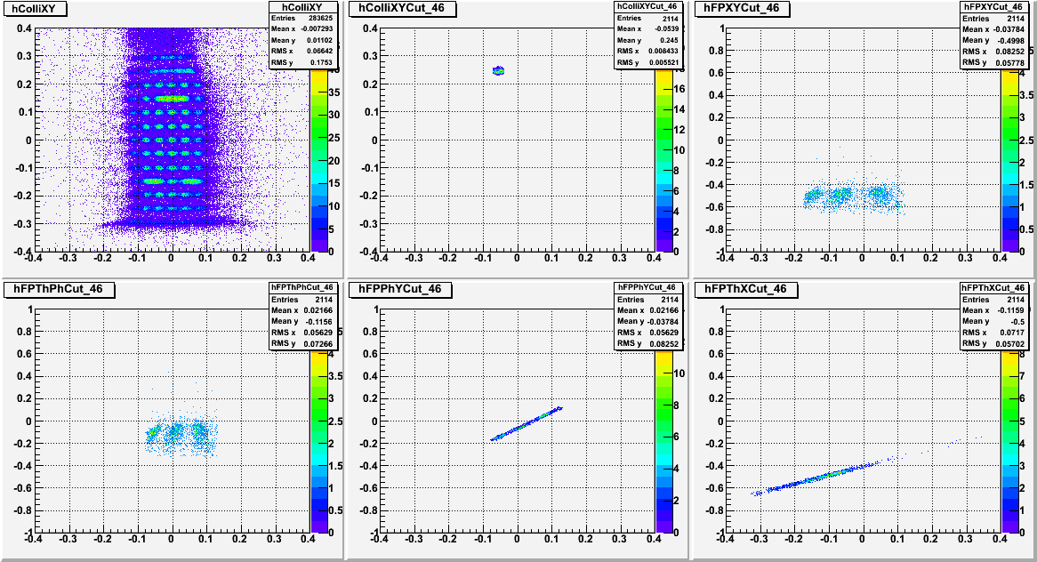
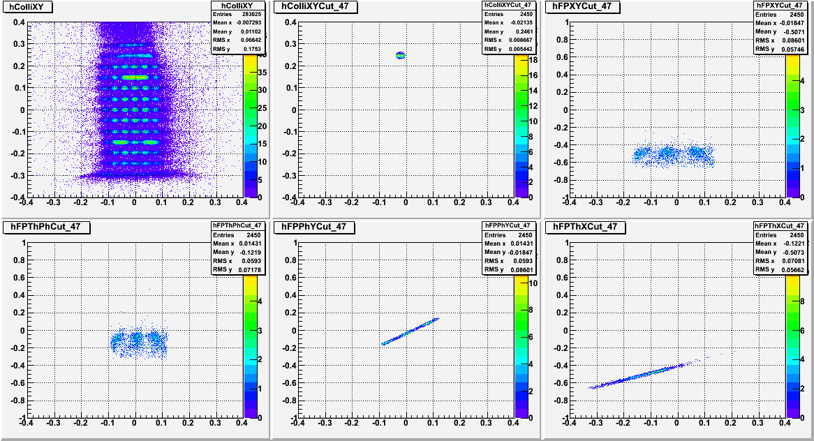
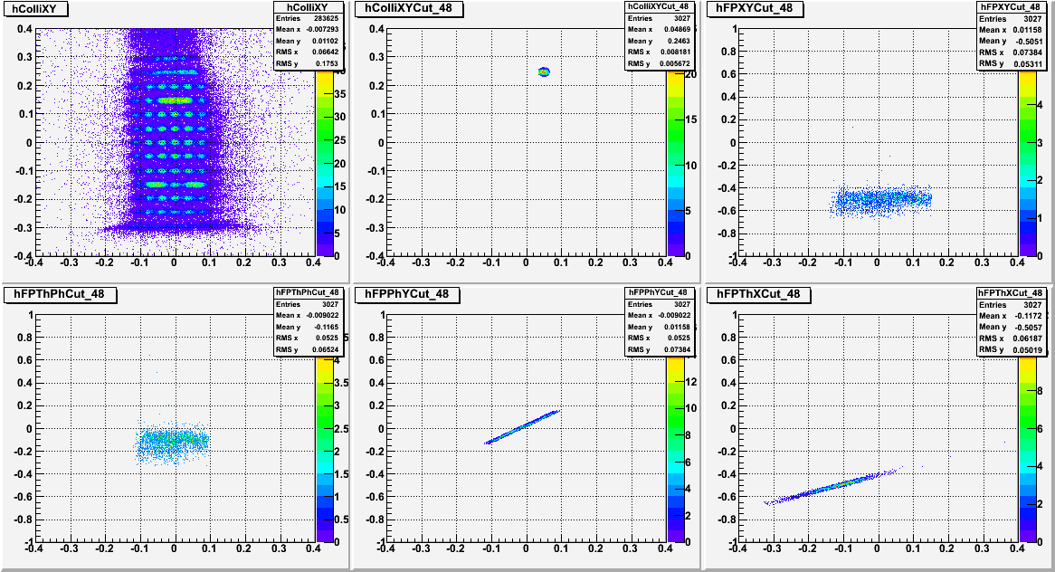
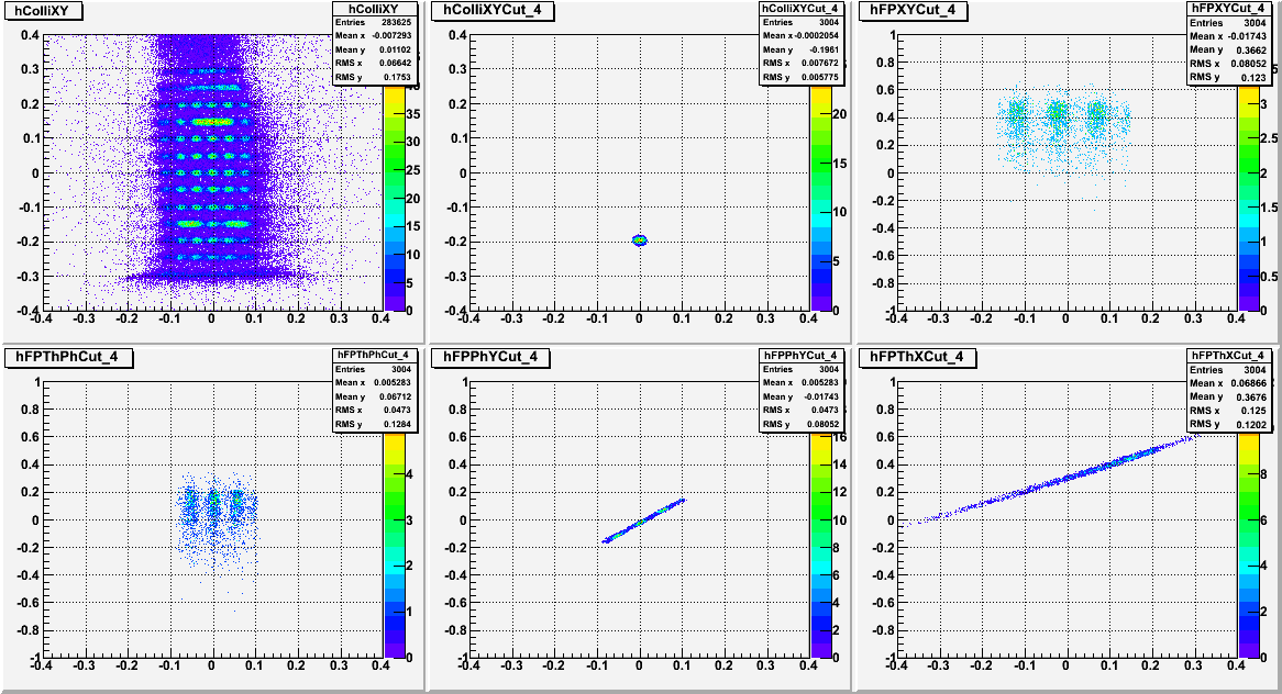
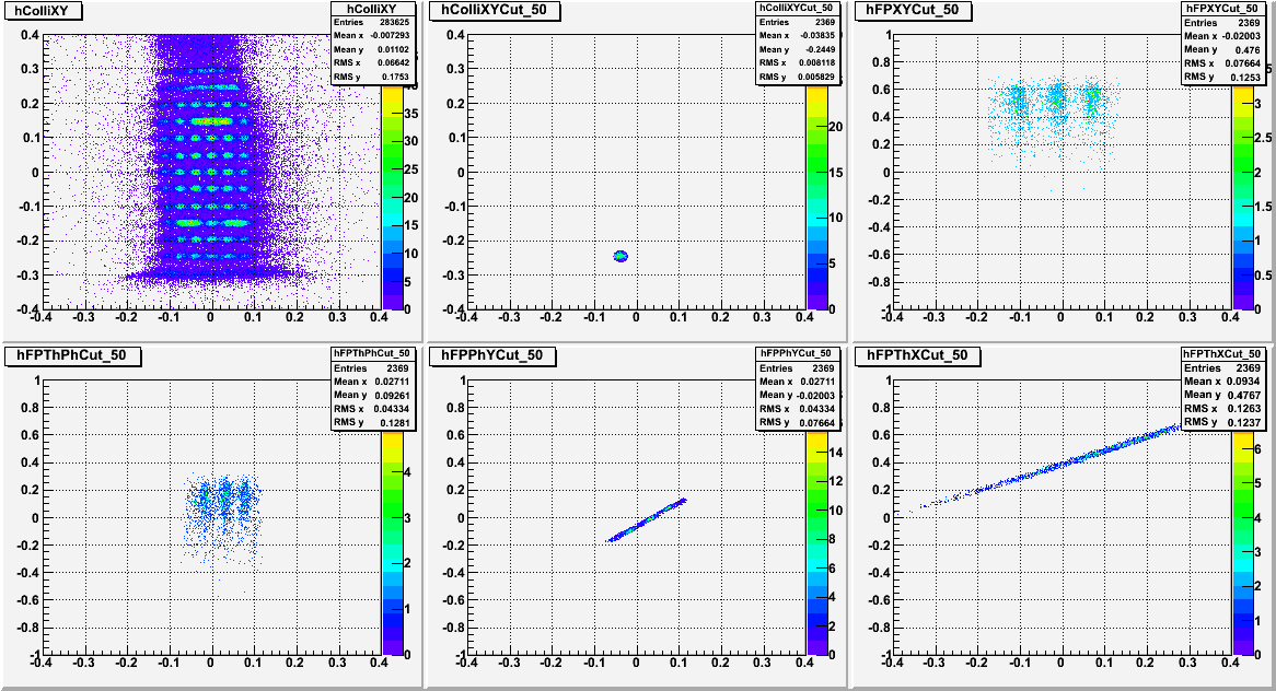
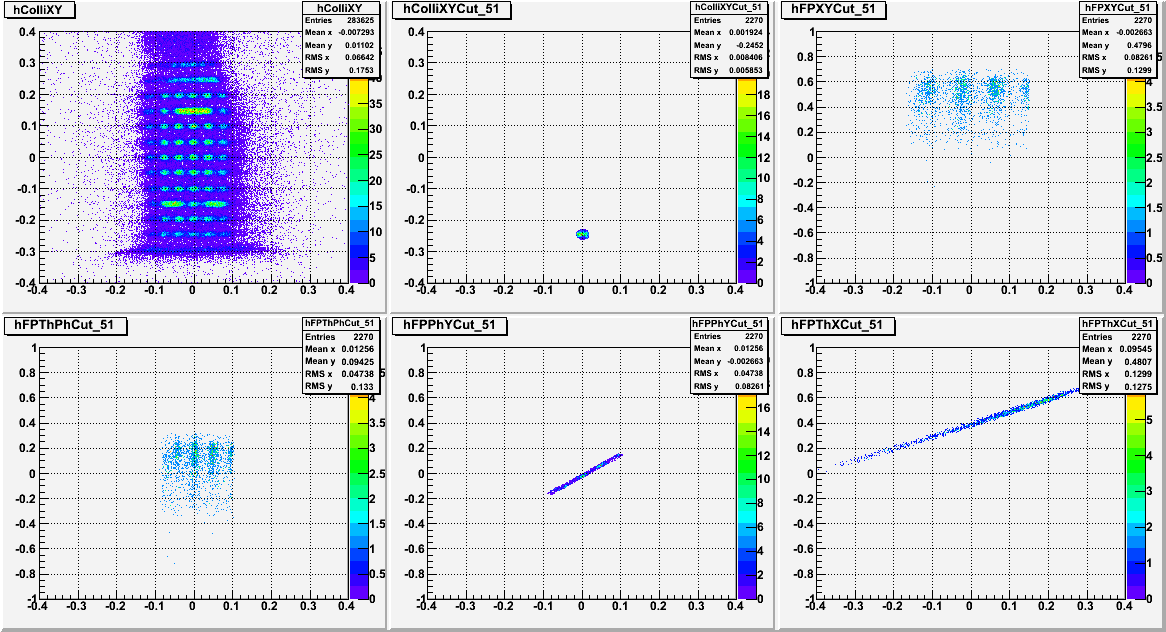
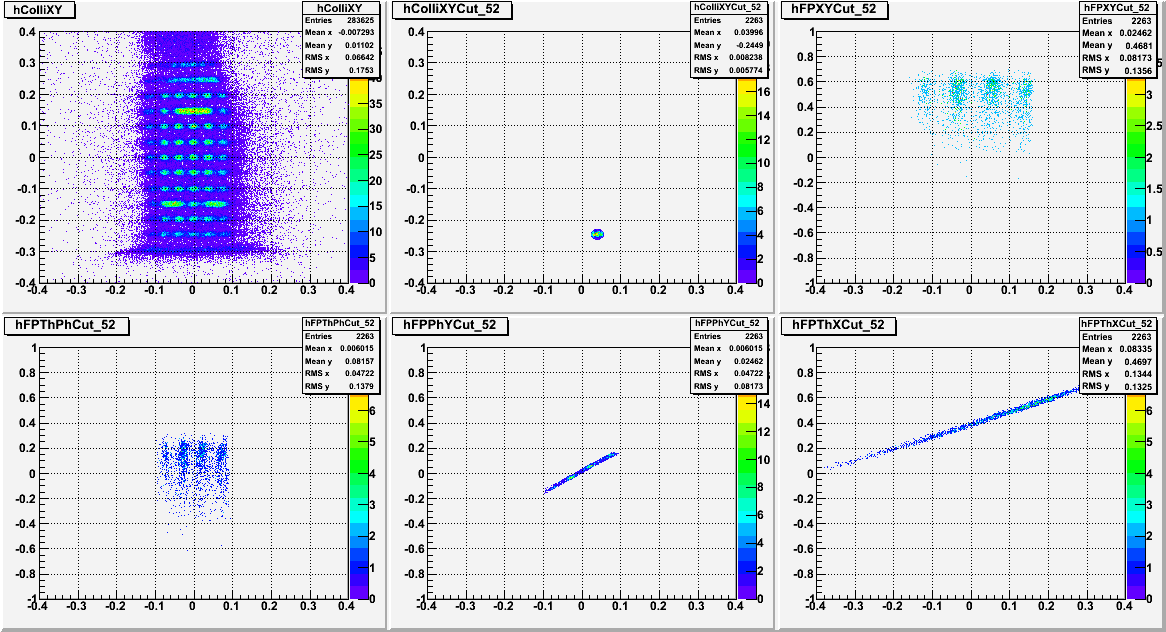
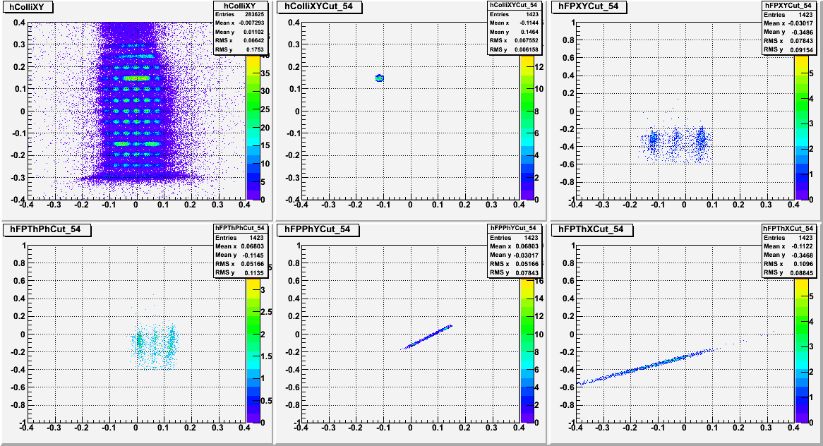
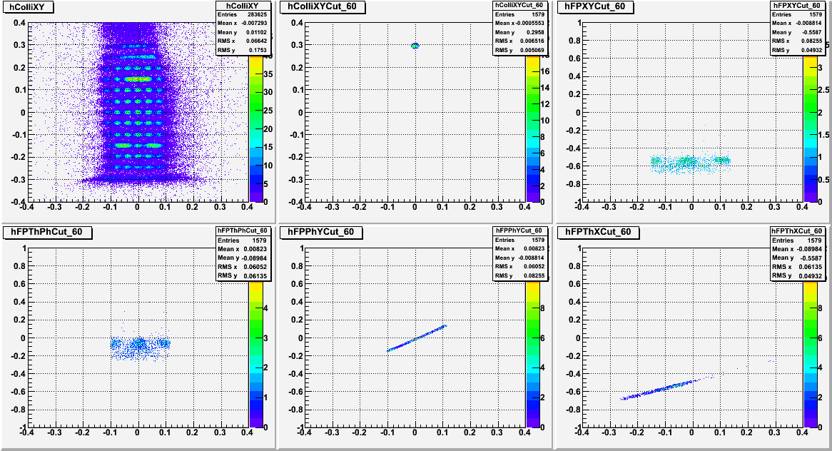
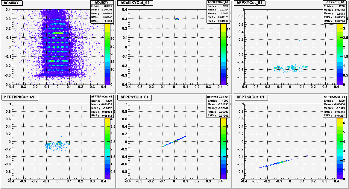
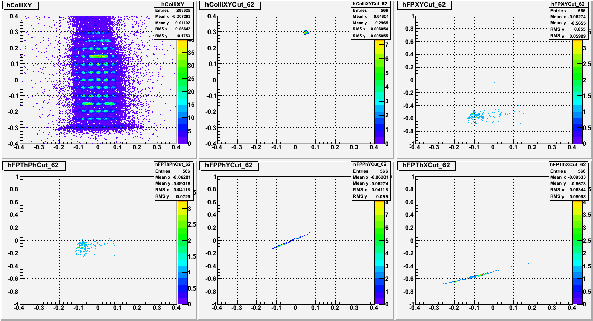
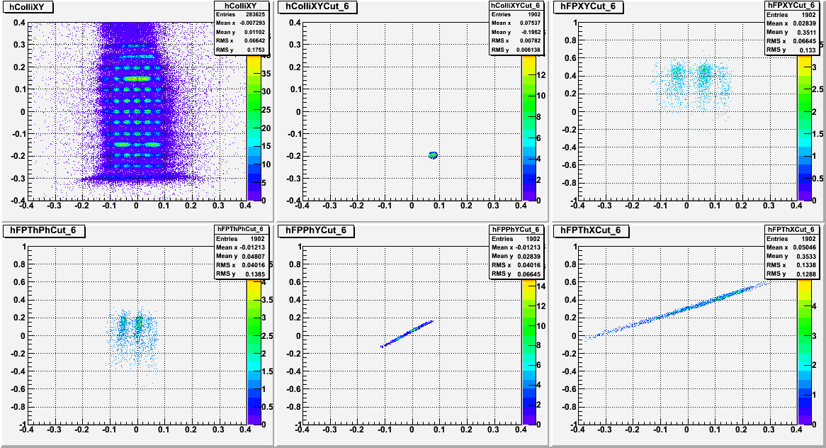
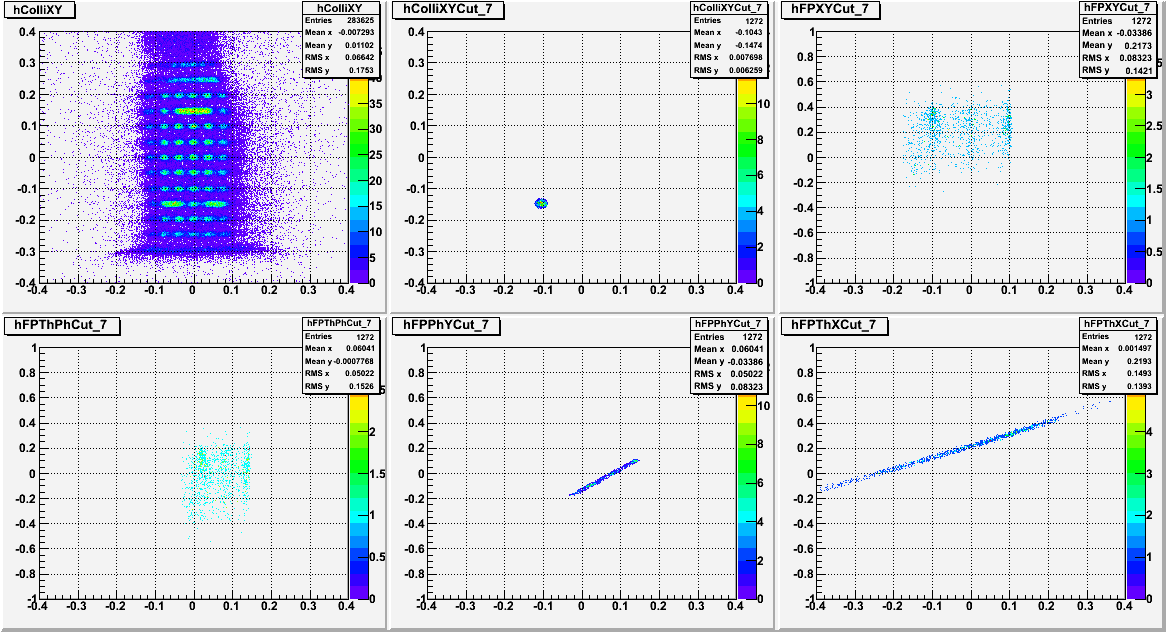
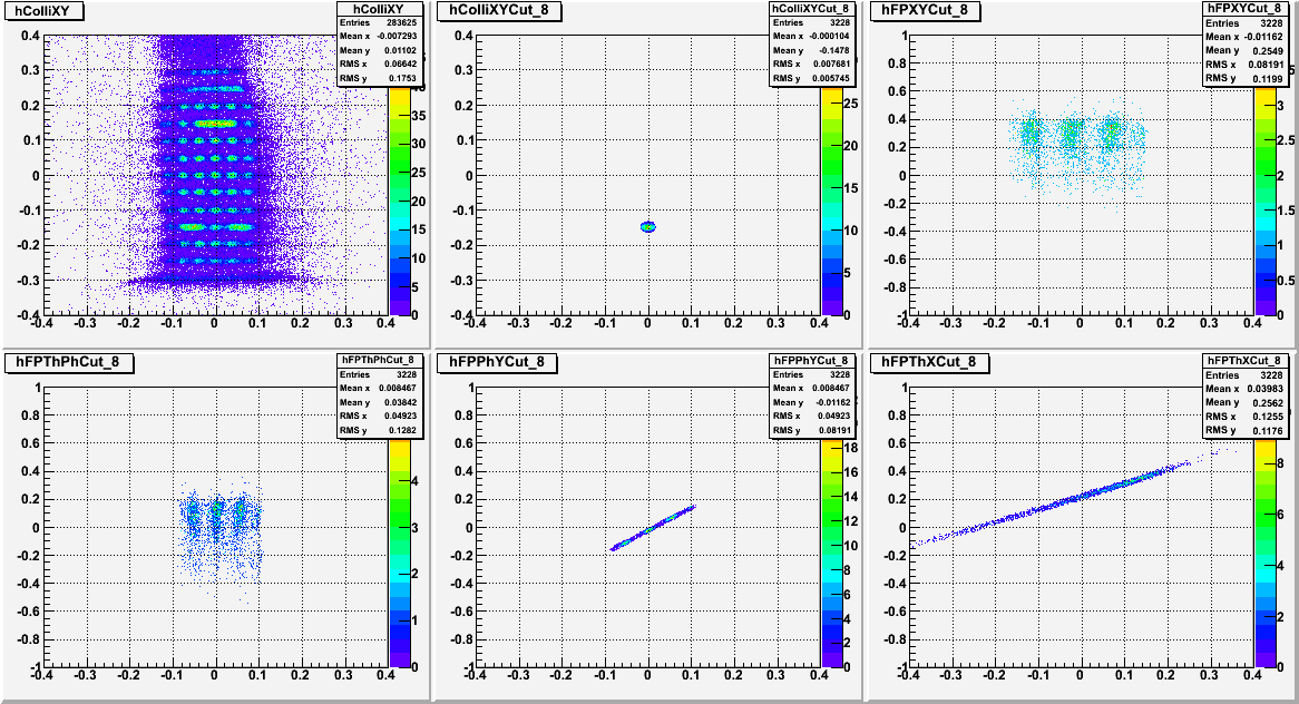
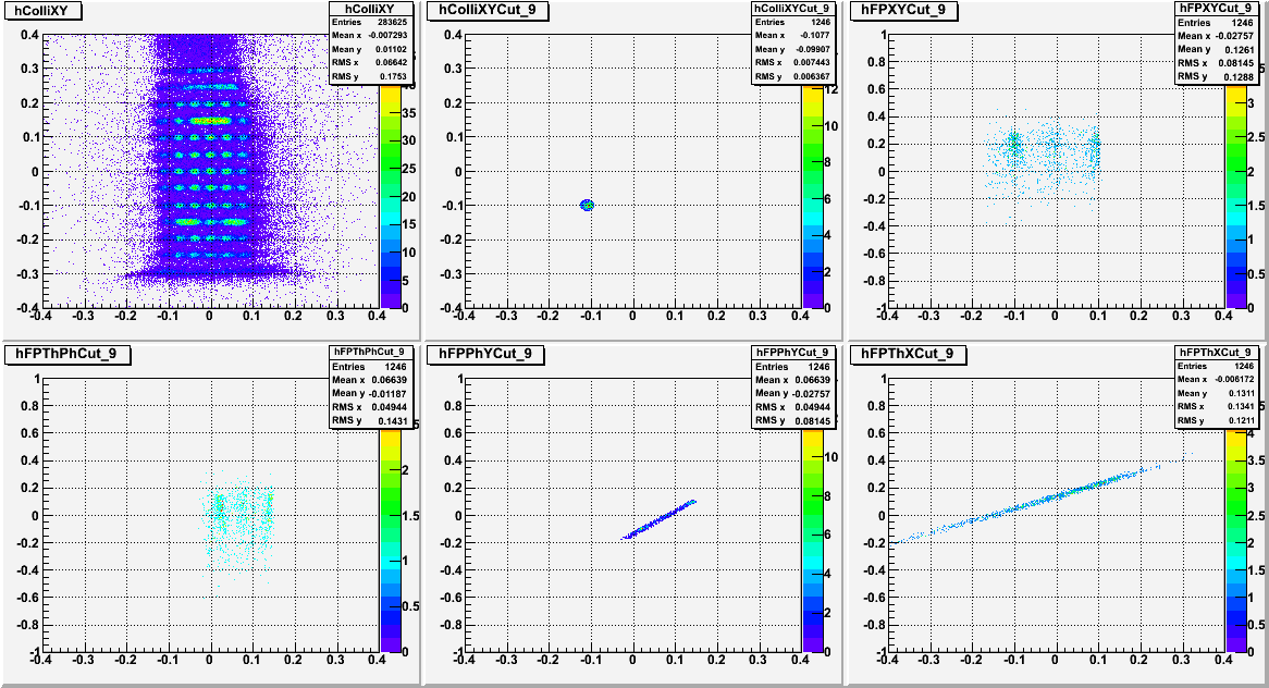
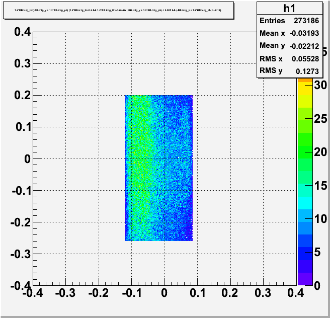
Figures show reconstructed sieve-pattern, that I get with current transport matrix.
3.)  4.)
4.) 
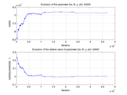
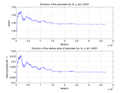
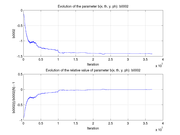
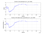
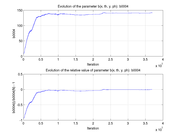
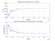
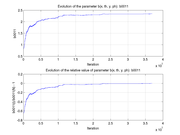
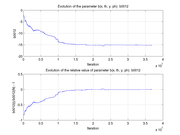
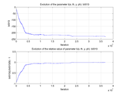
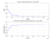
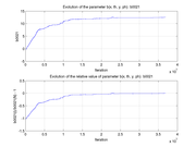
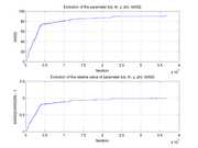
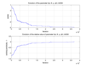
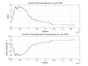
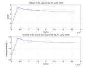
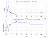
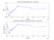
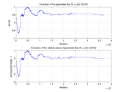
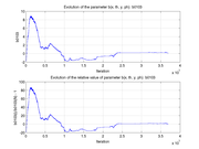
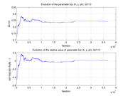
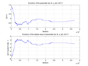
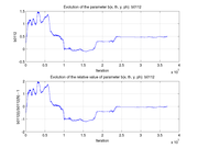
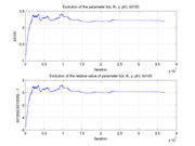
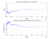
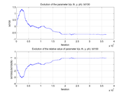
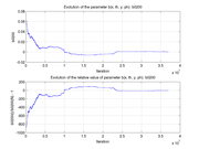
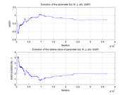
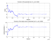
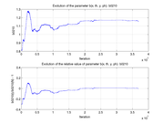
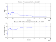
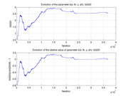
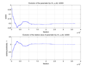
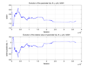
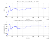
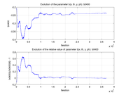
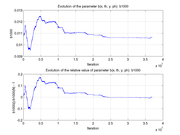
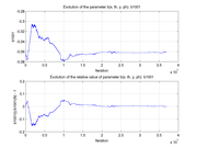
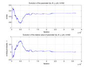
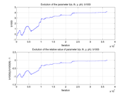
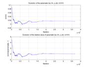
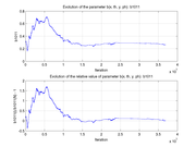
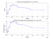
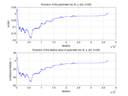
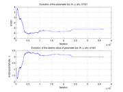
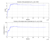
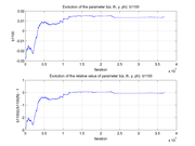
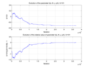
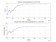
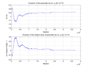
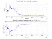
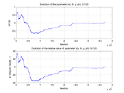
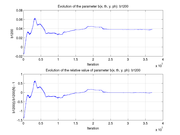
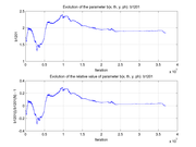
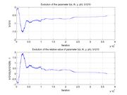
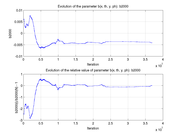
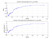
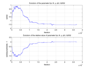
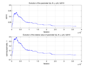
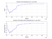
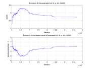
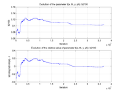
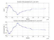
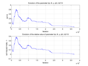
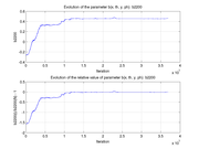
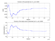
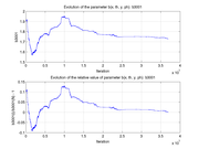
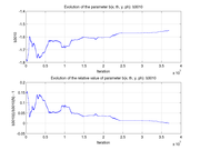
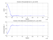
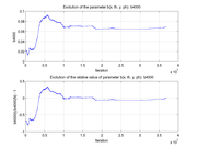
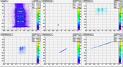
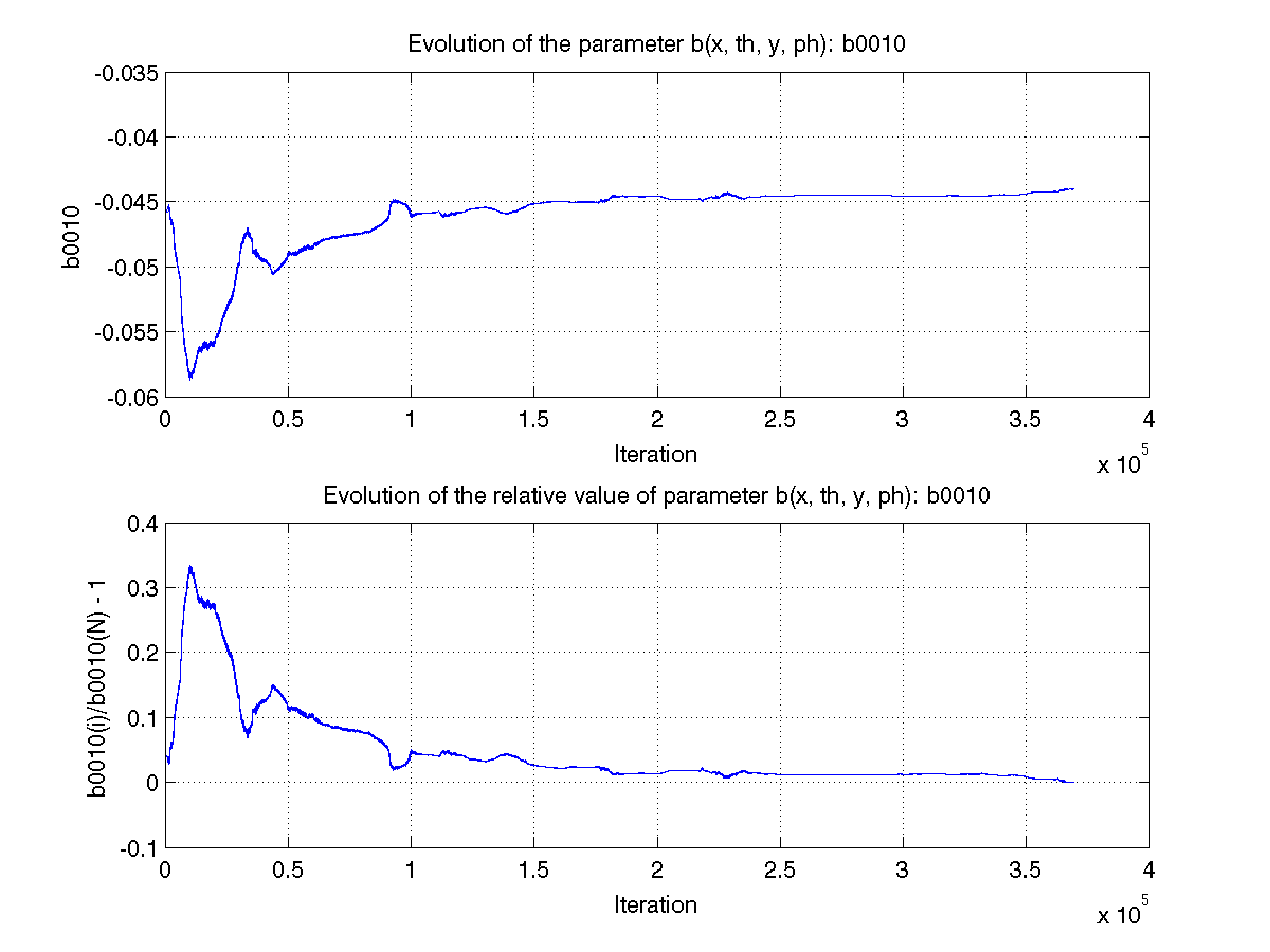
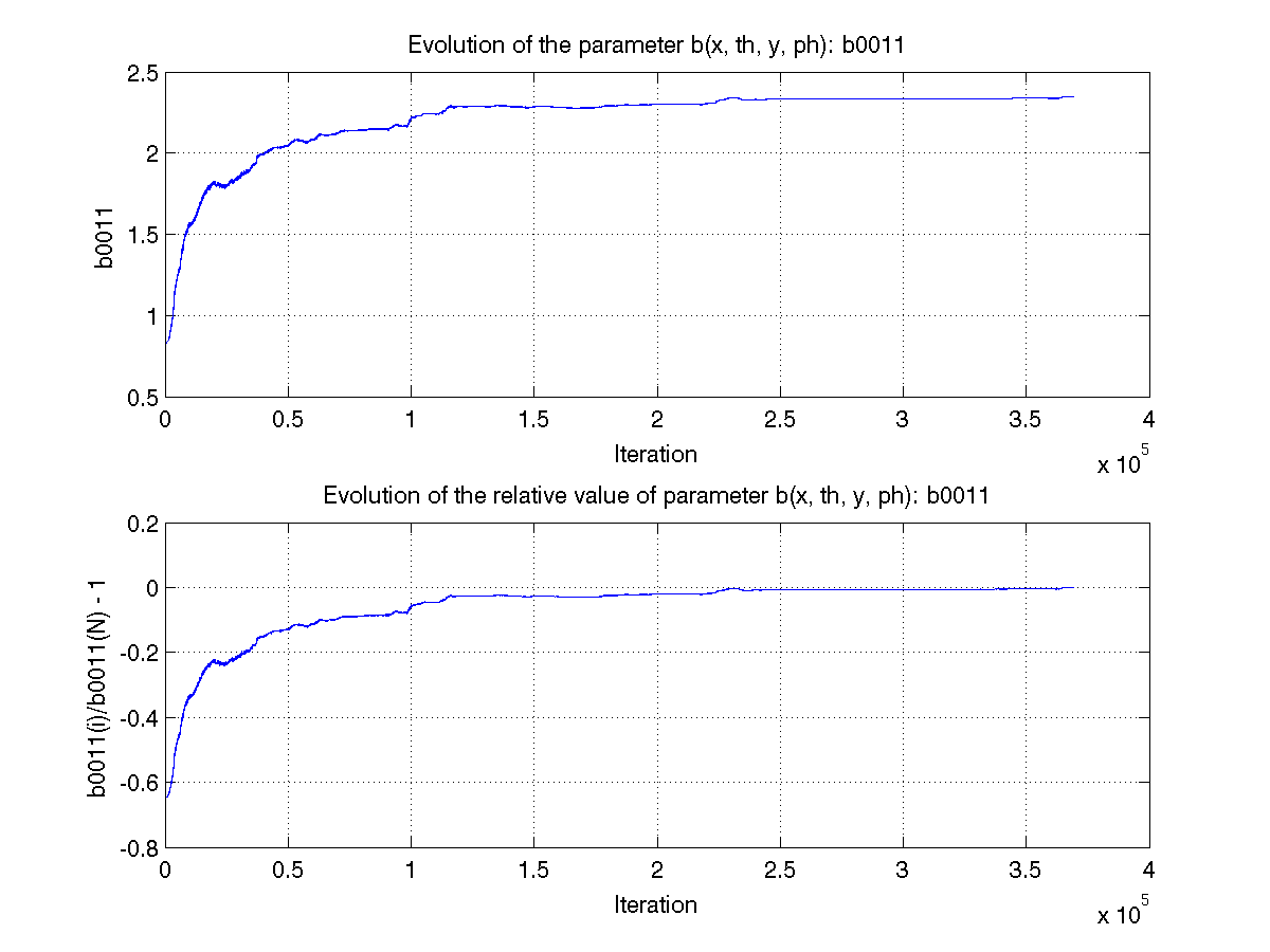
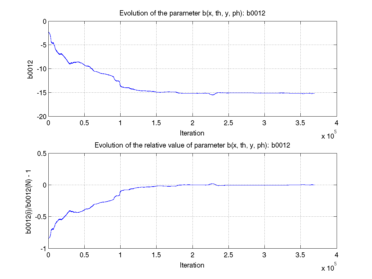
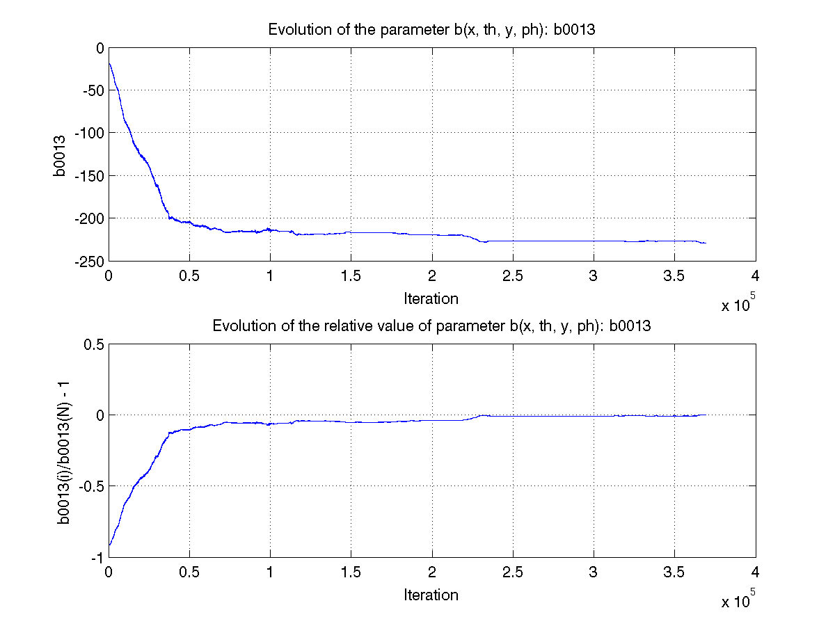
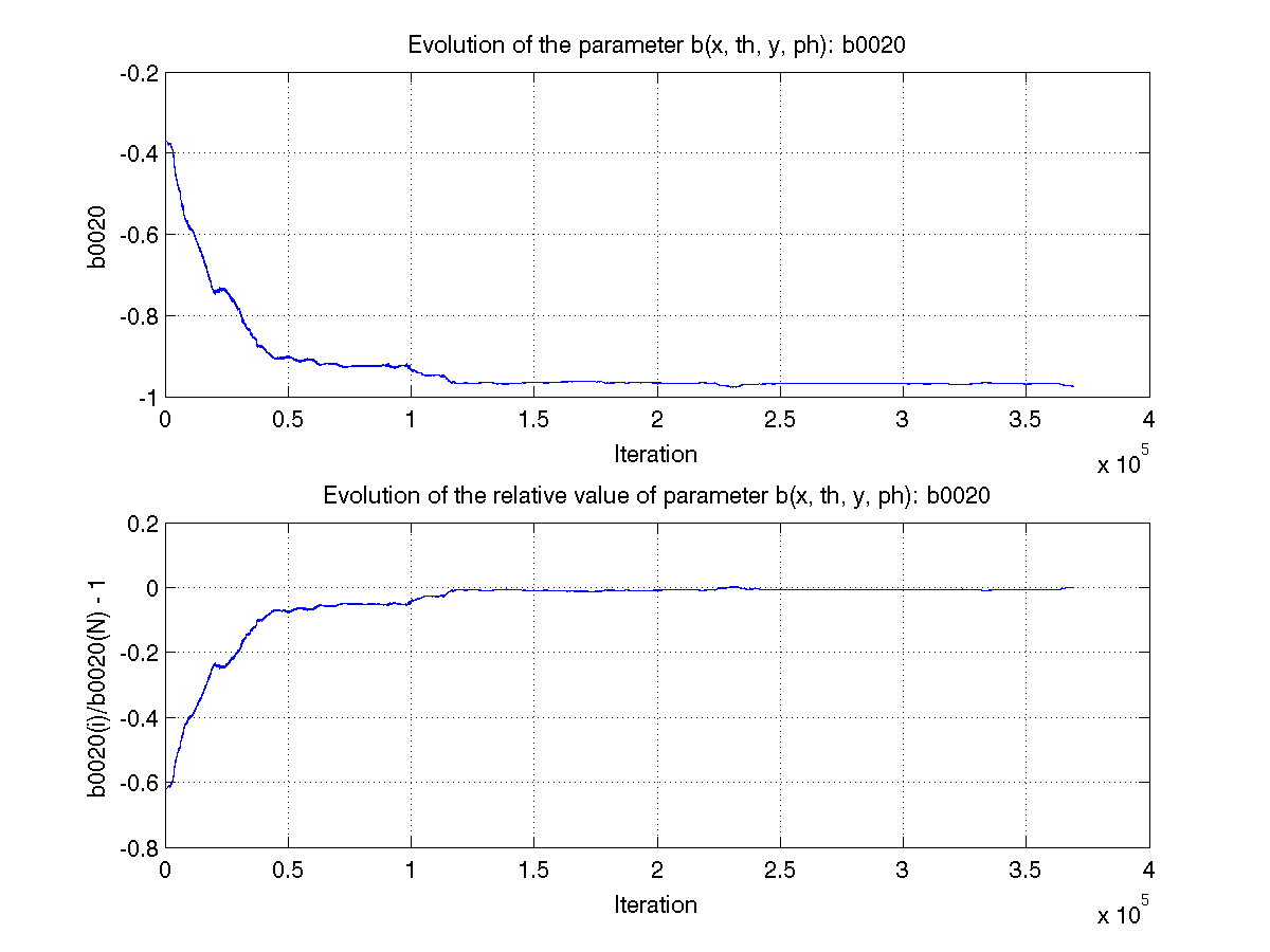
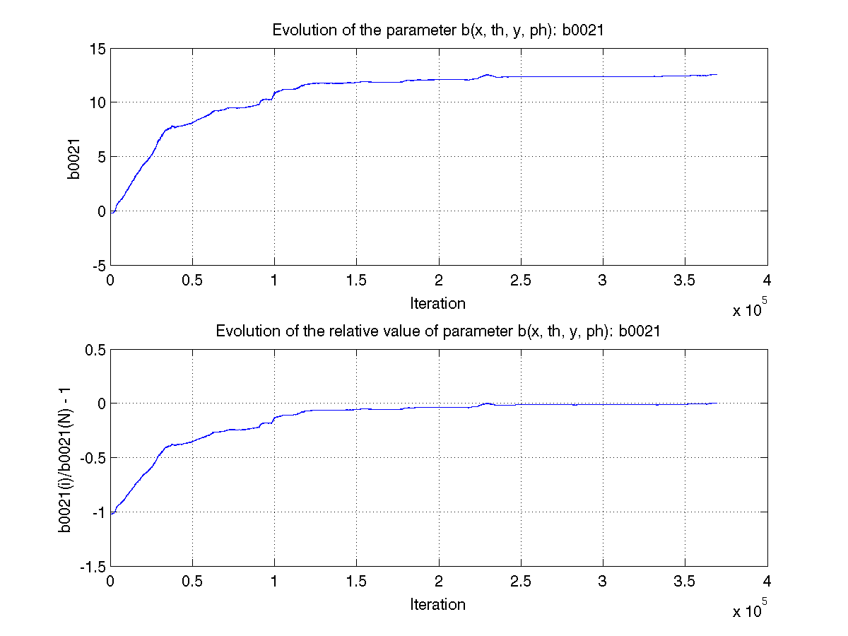
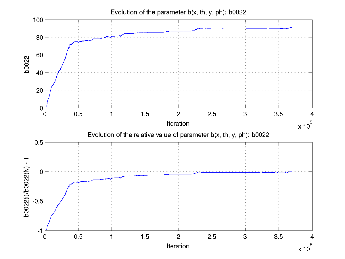
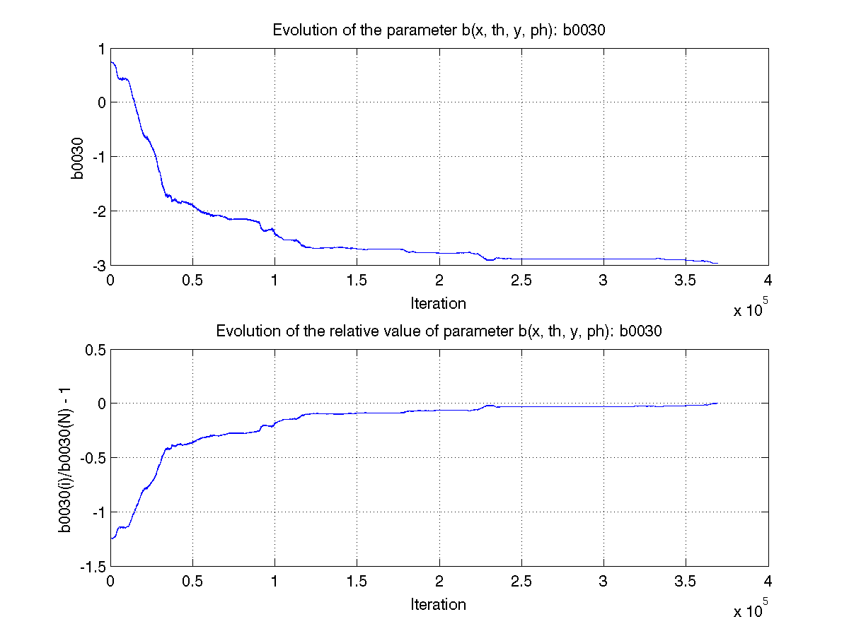
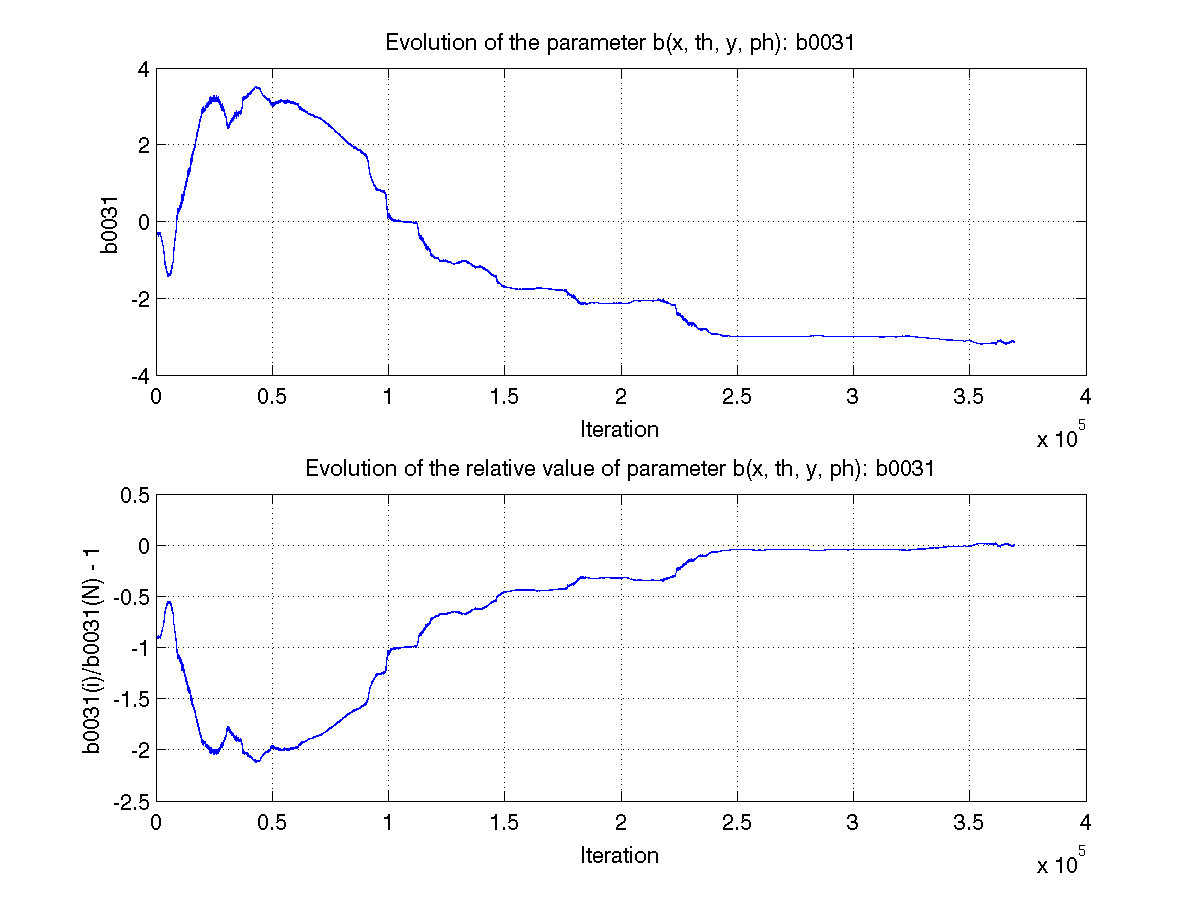
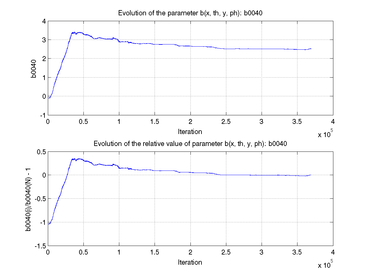
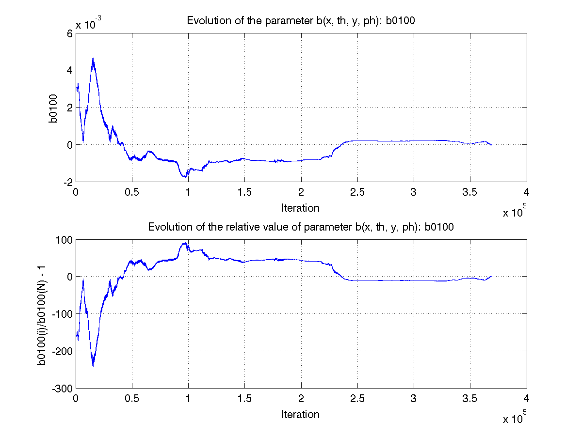
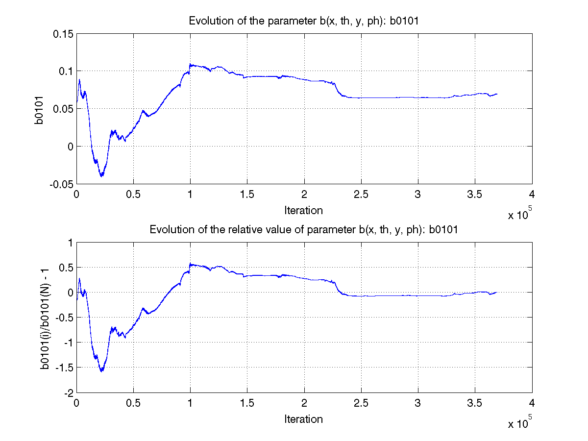
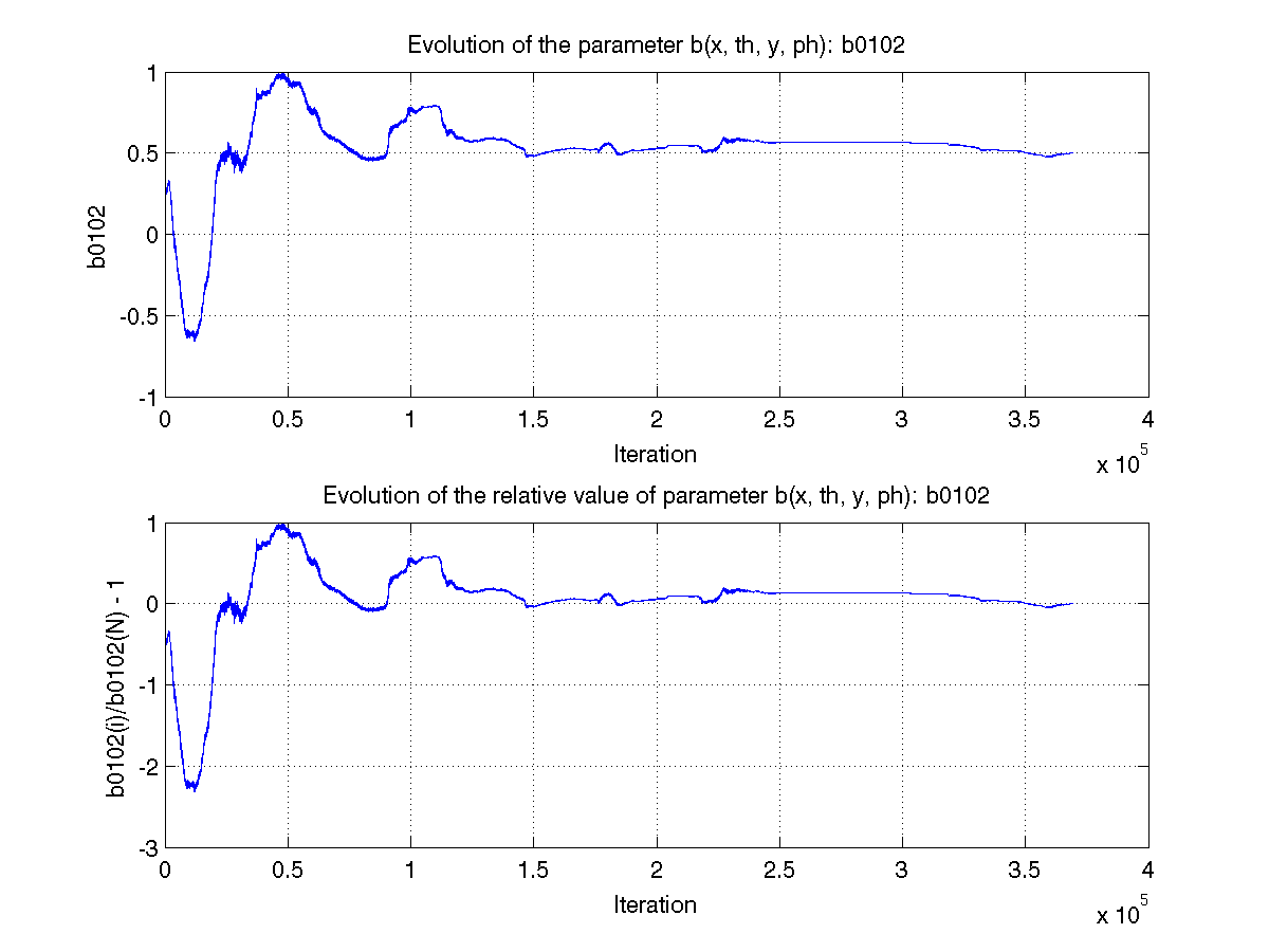
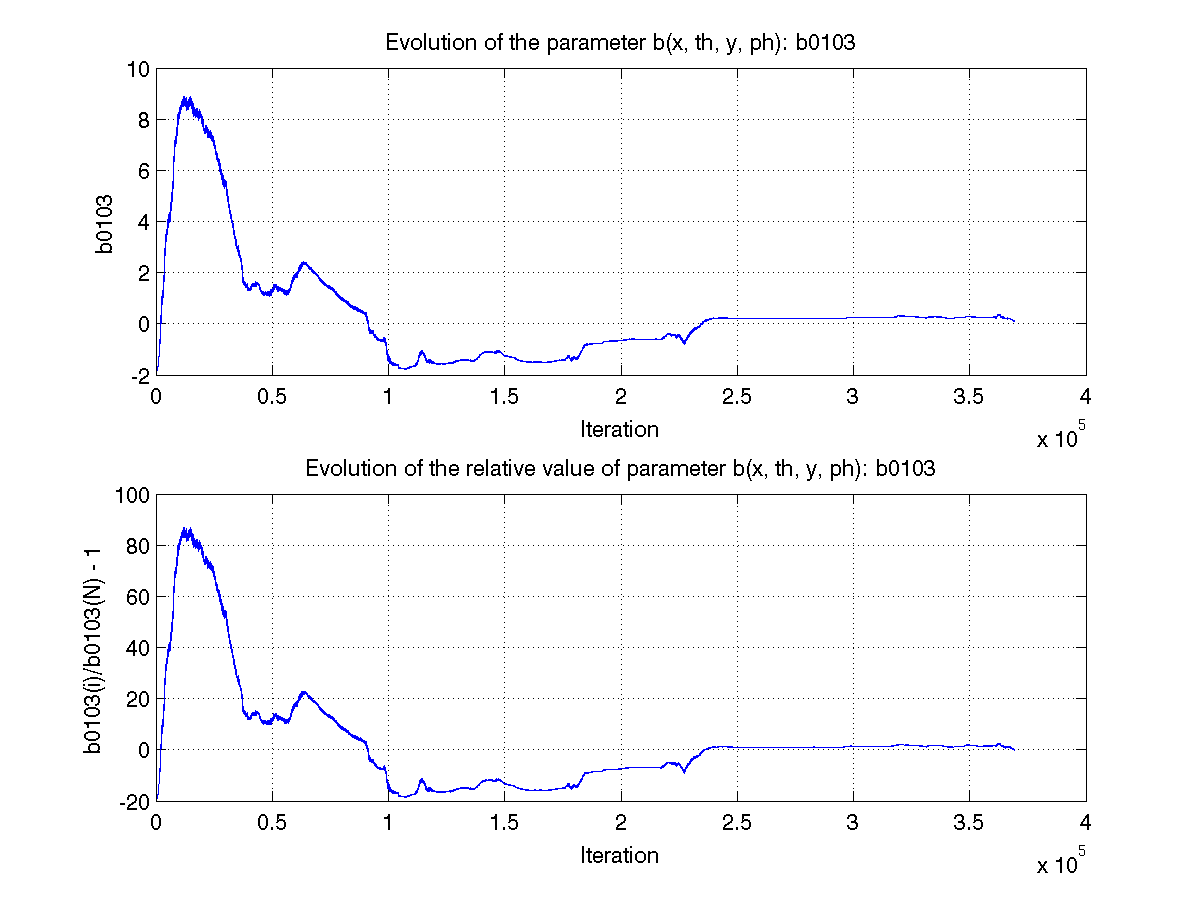
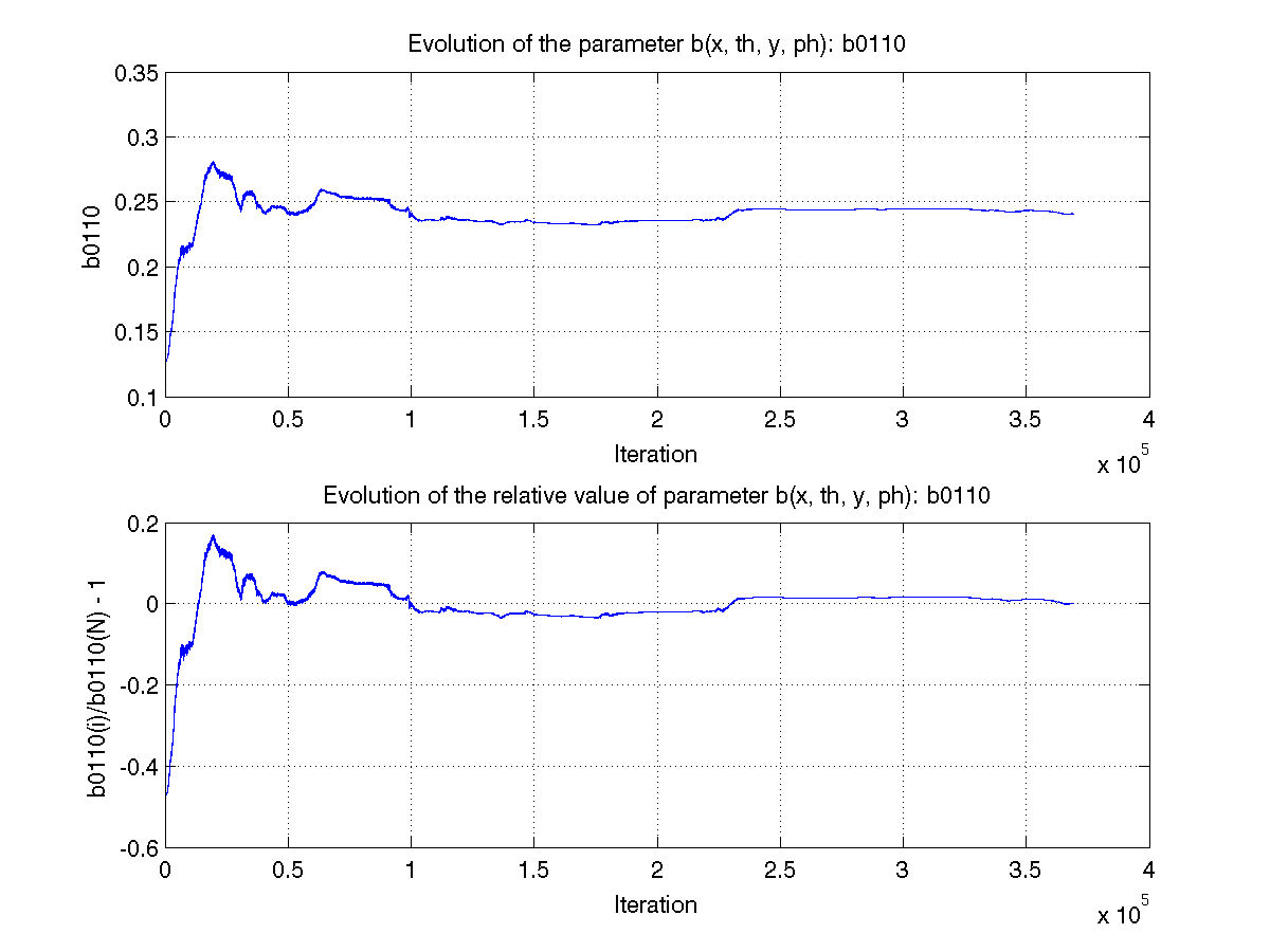
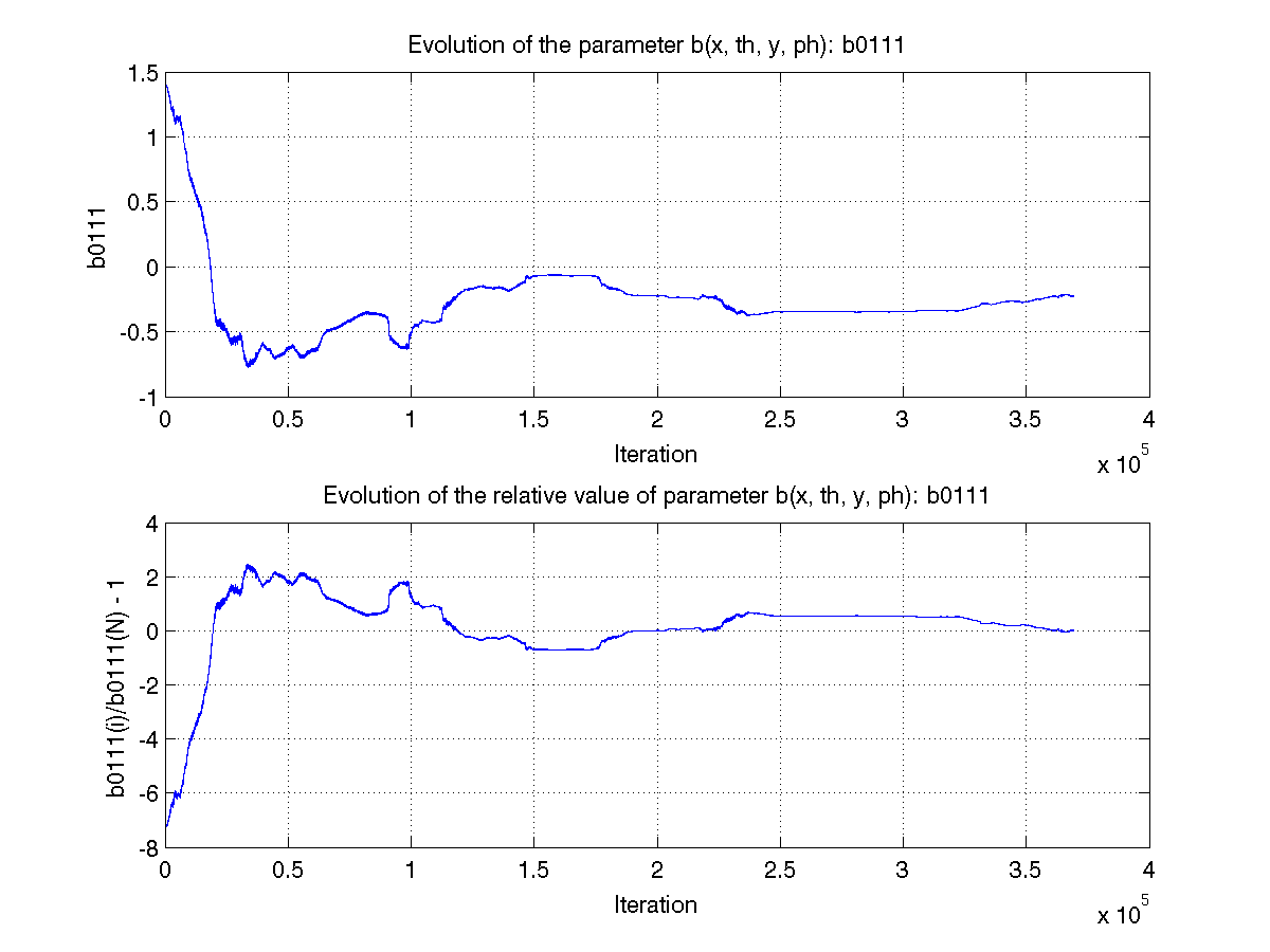
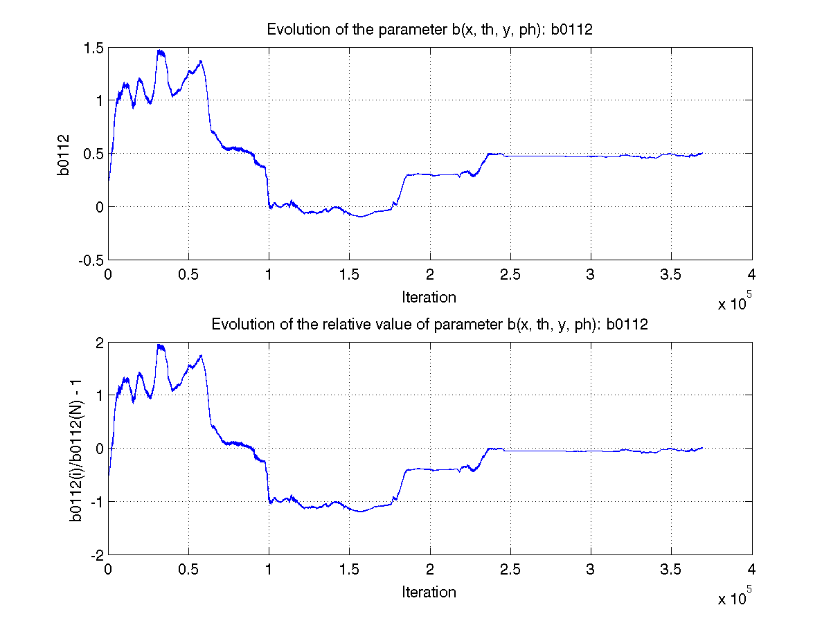
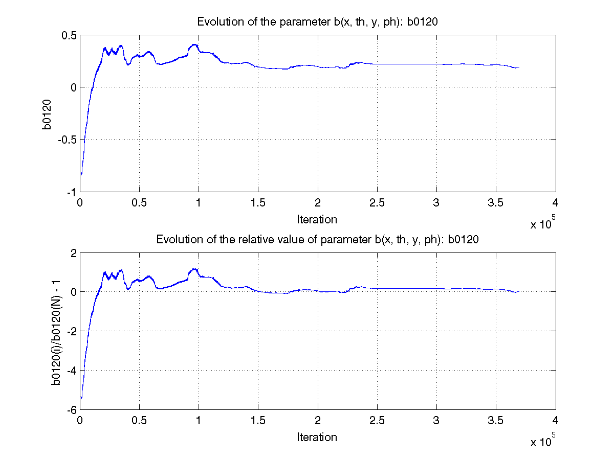
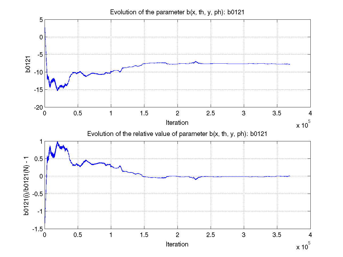
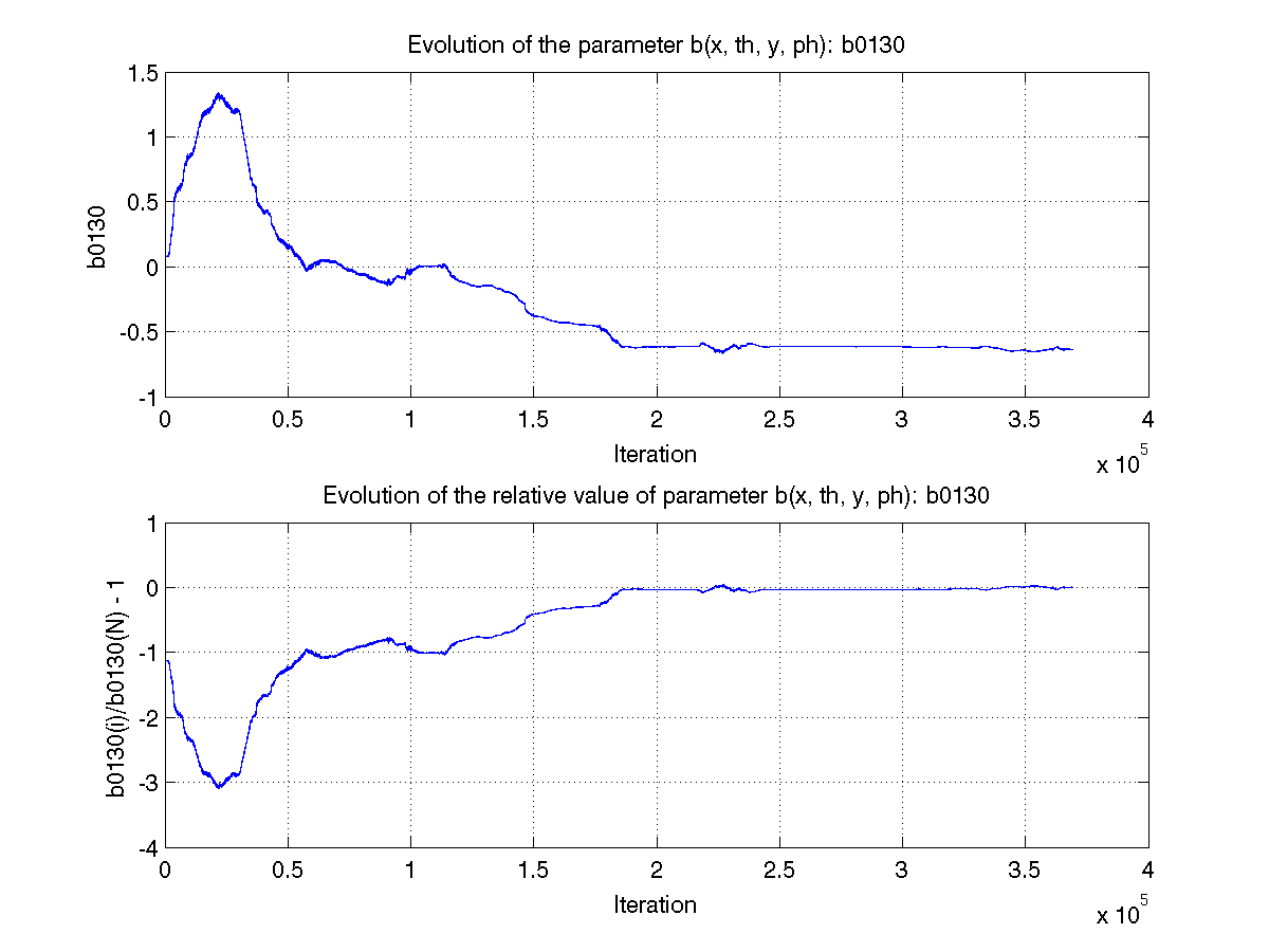
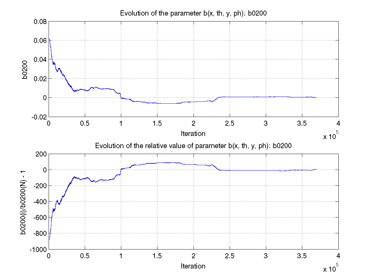
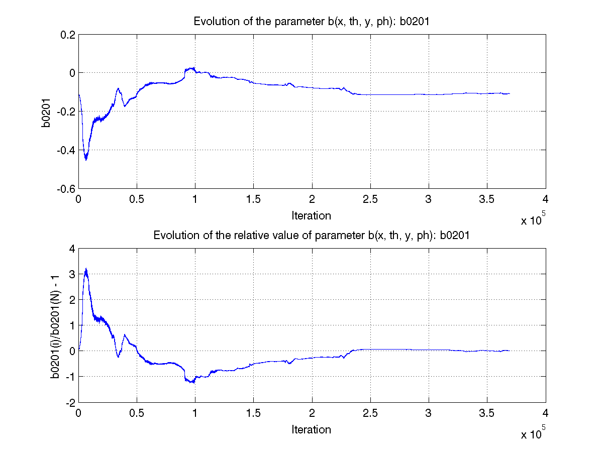
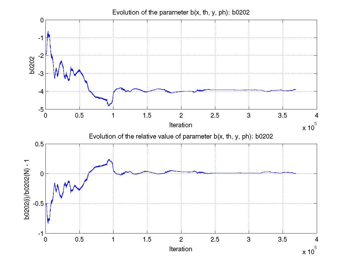
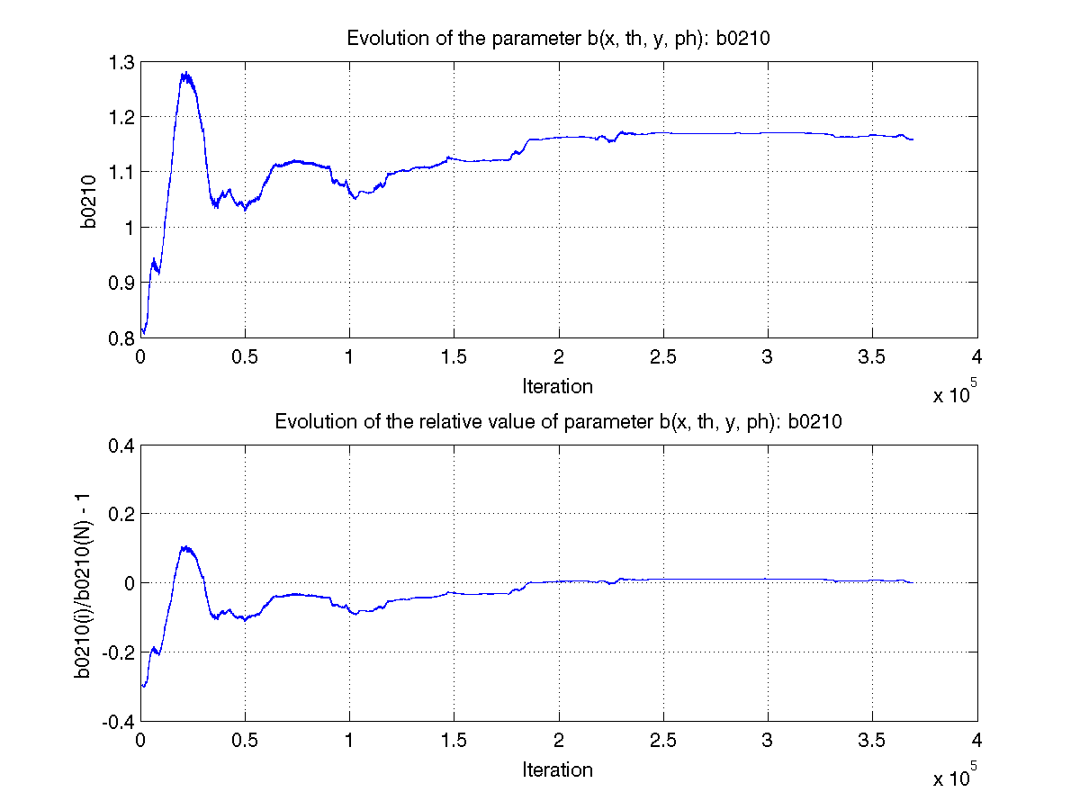
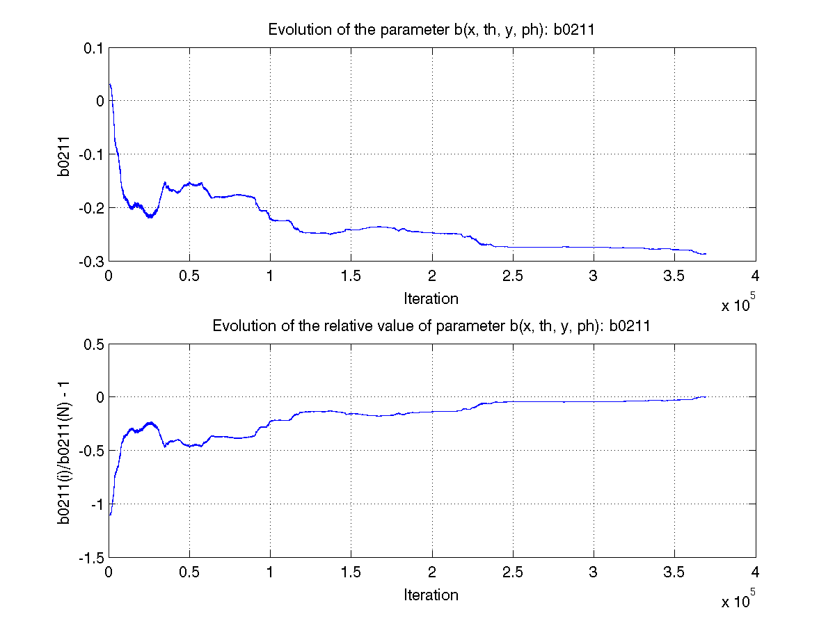
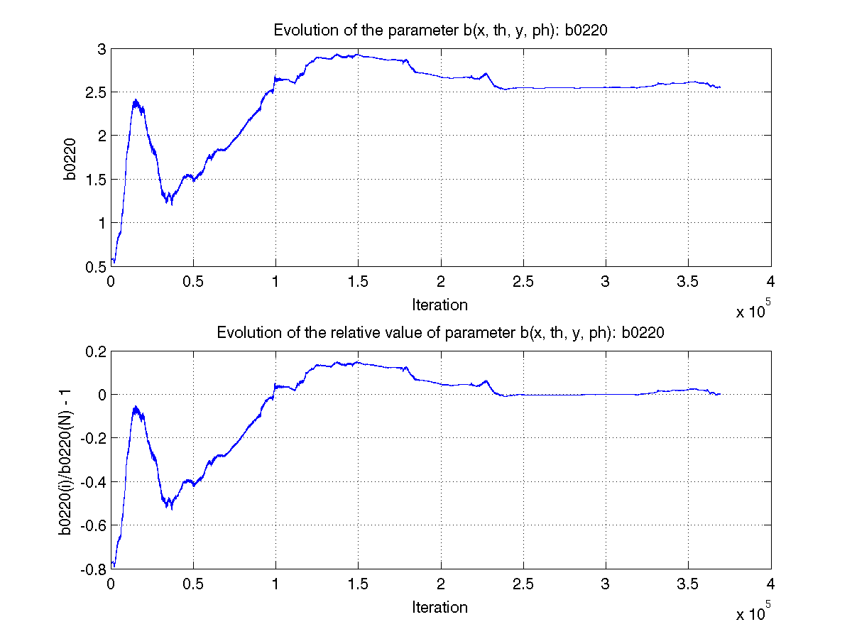
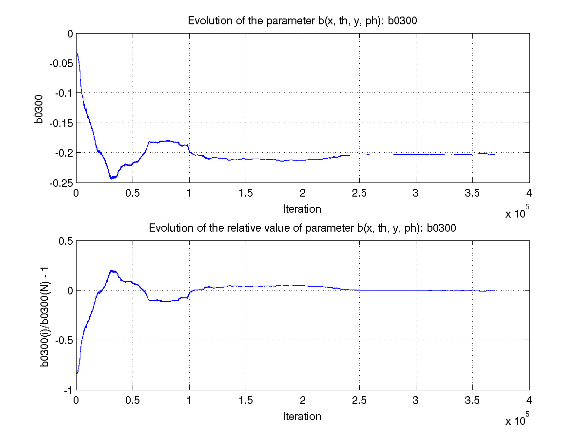
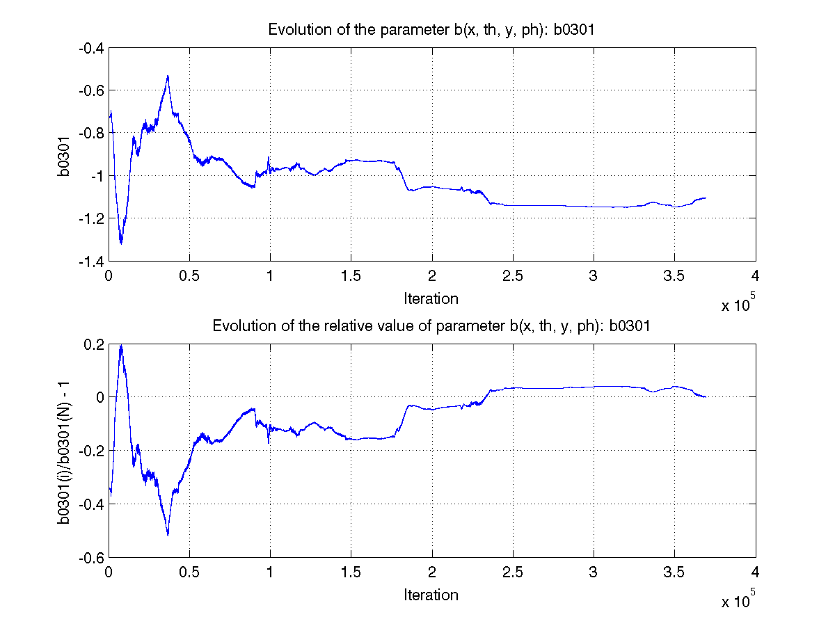
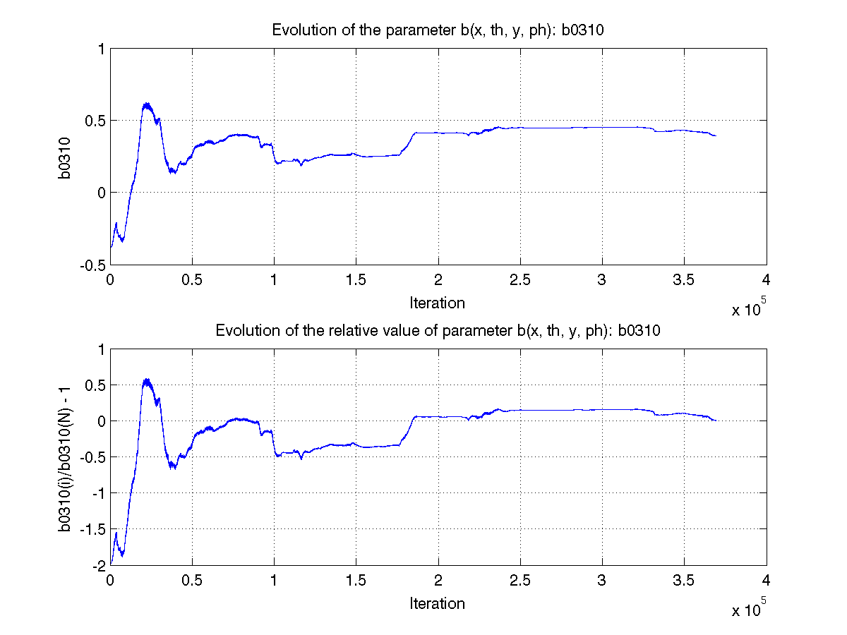
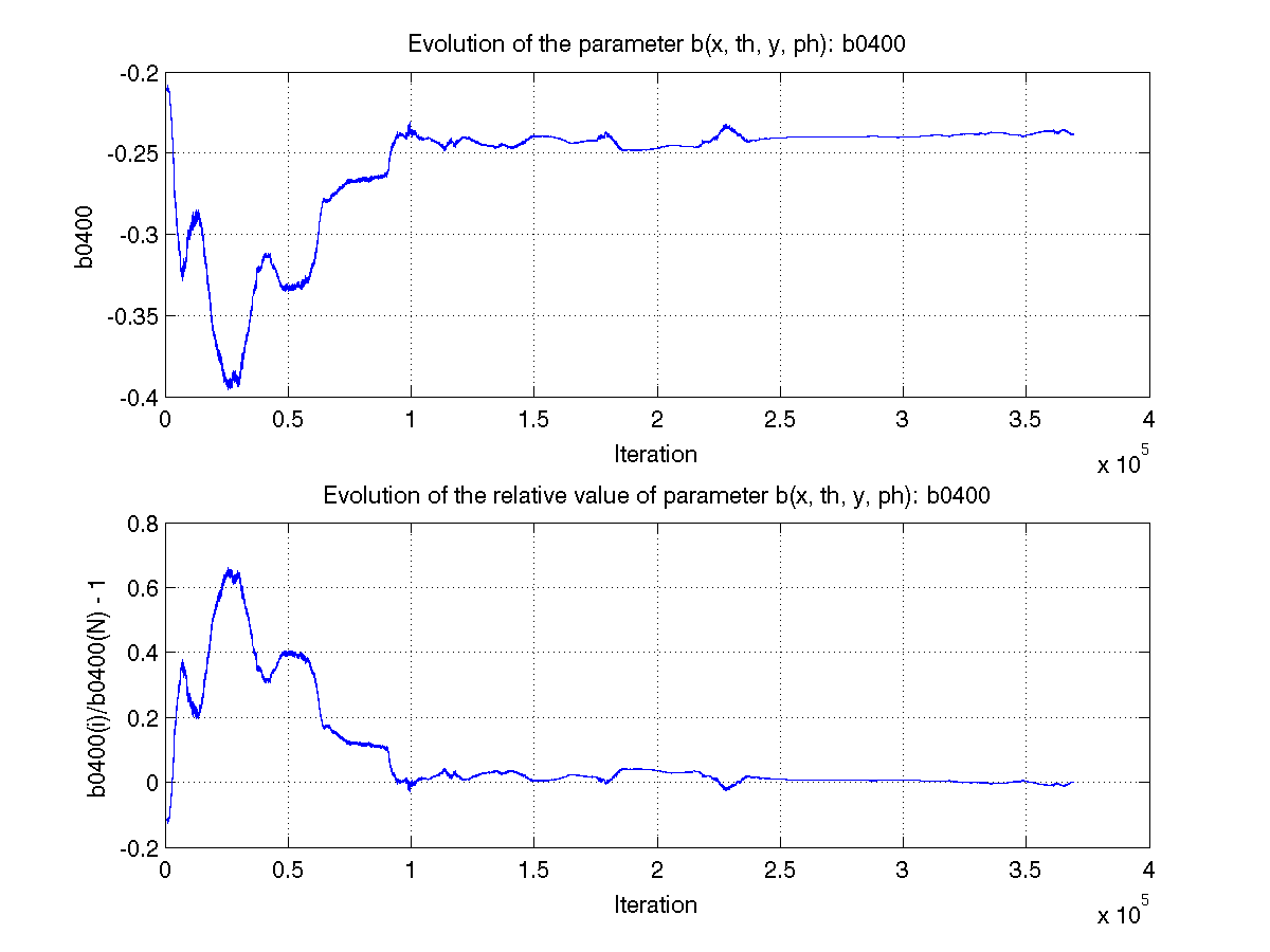
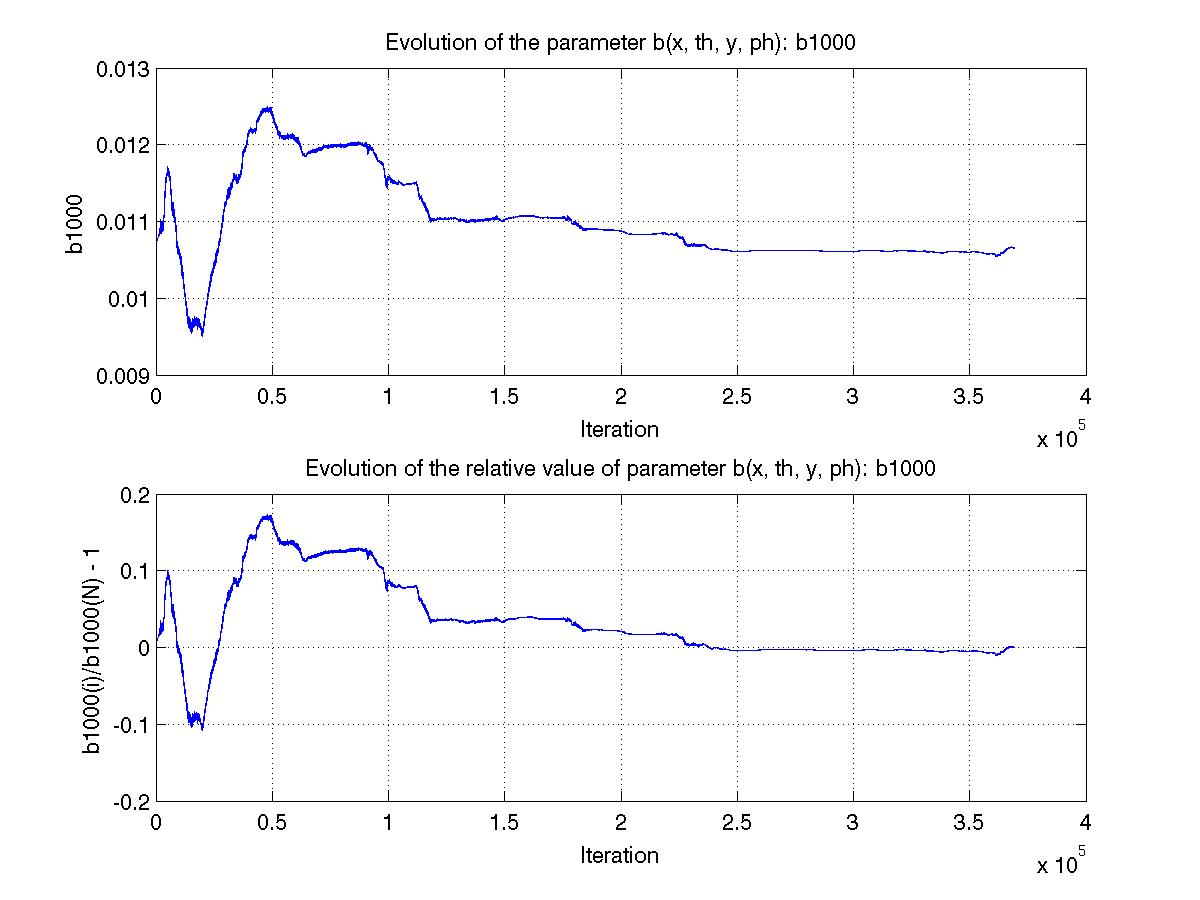
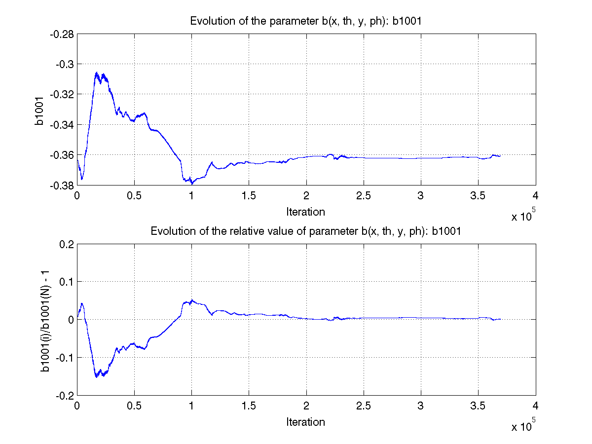
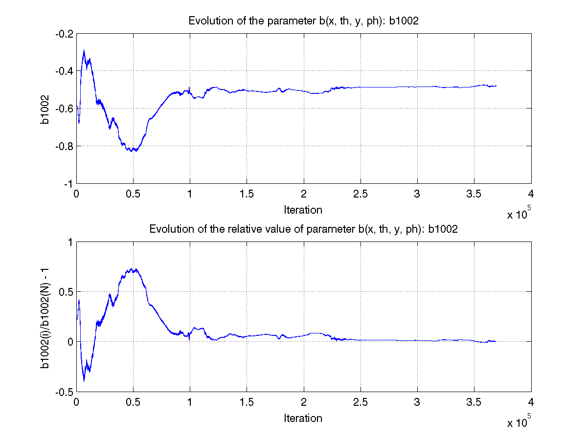
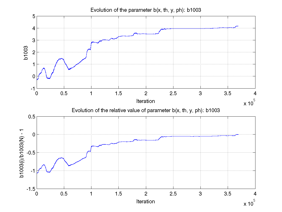
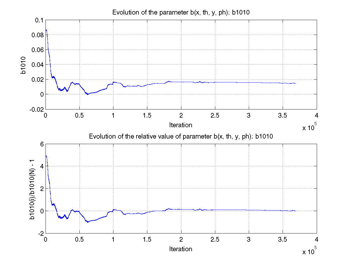
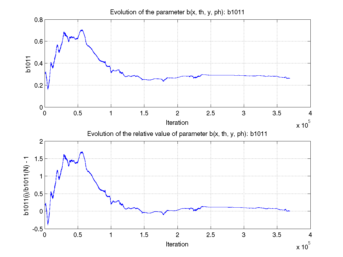
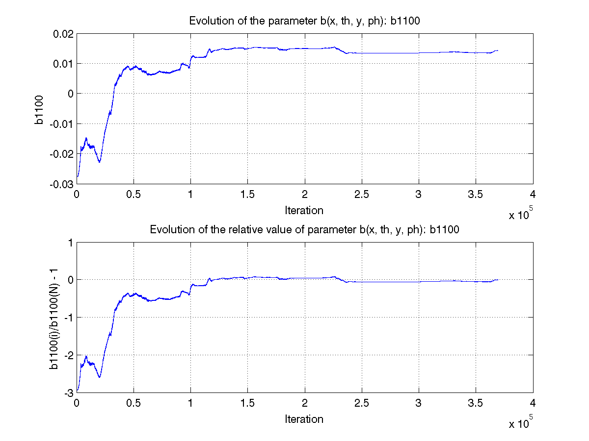
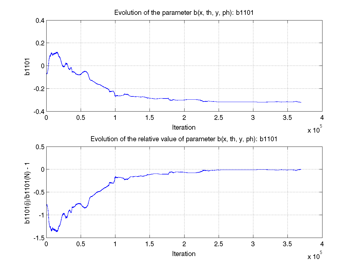
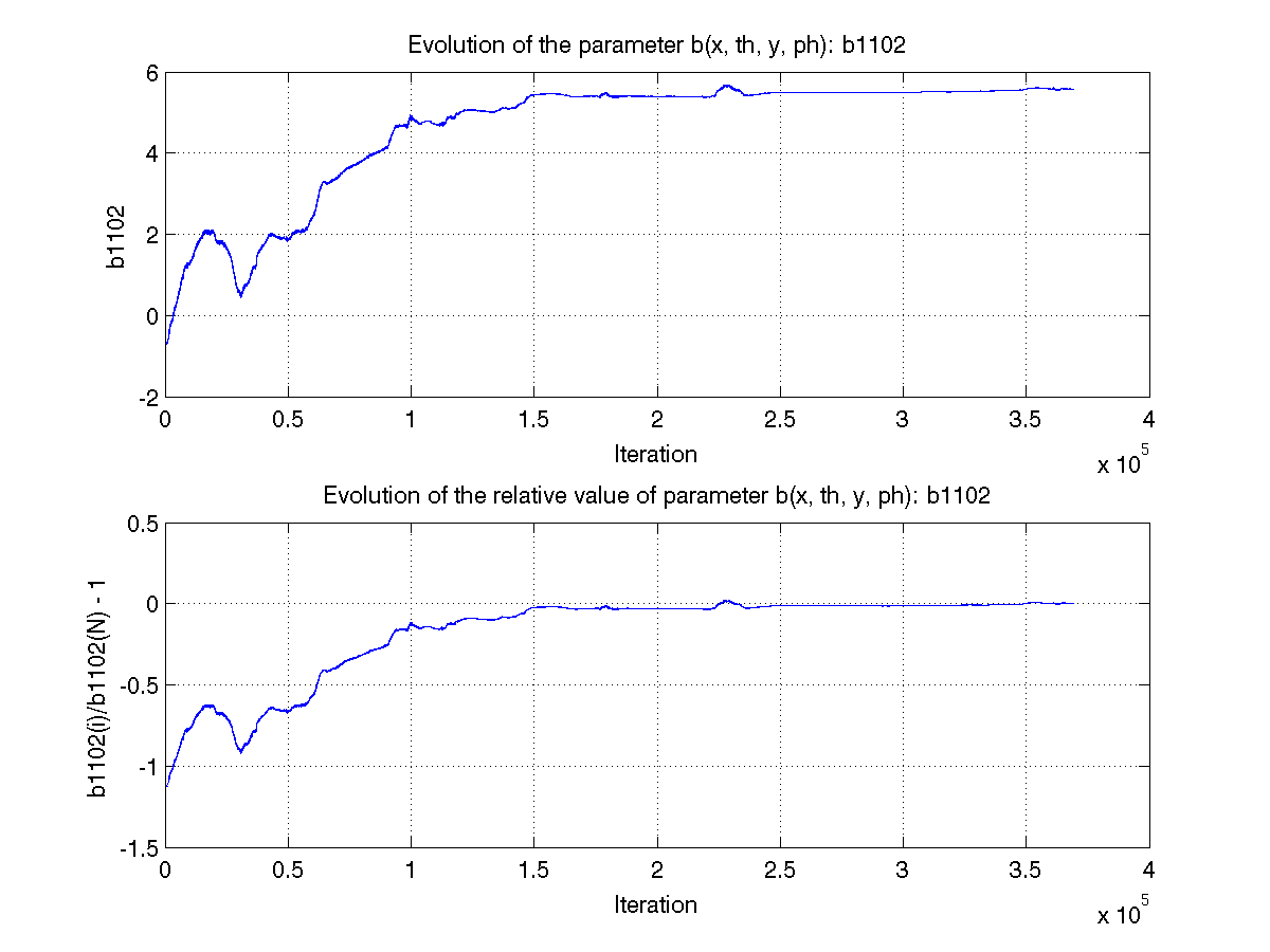
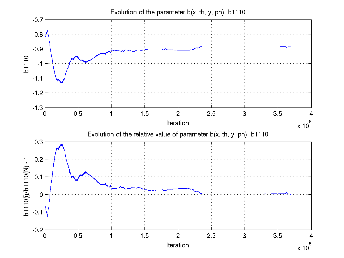
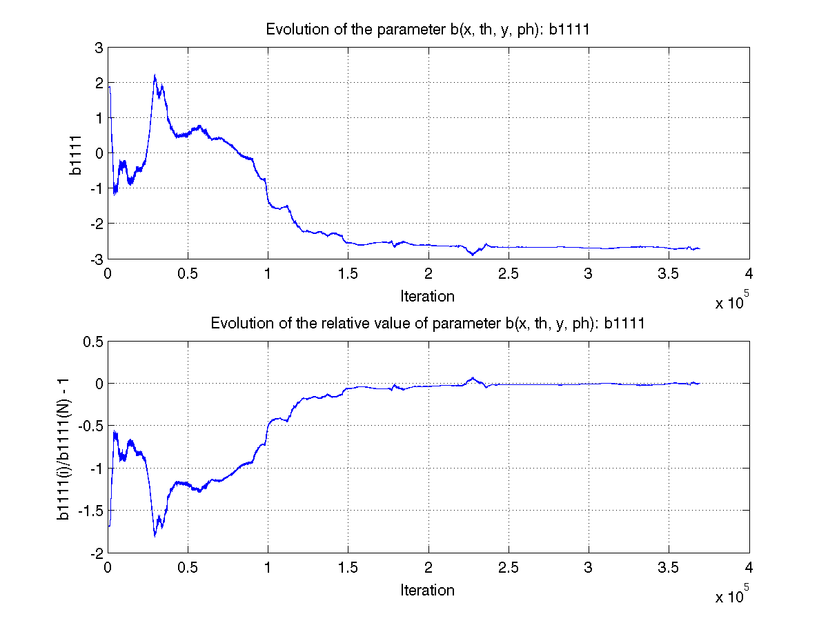
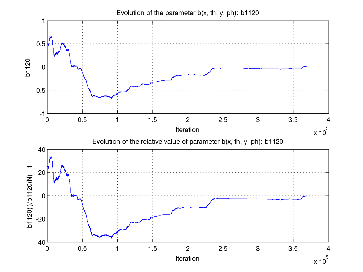
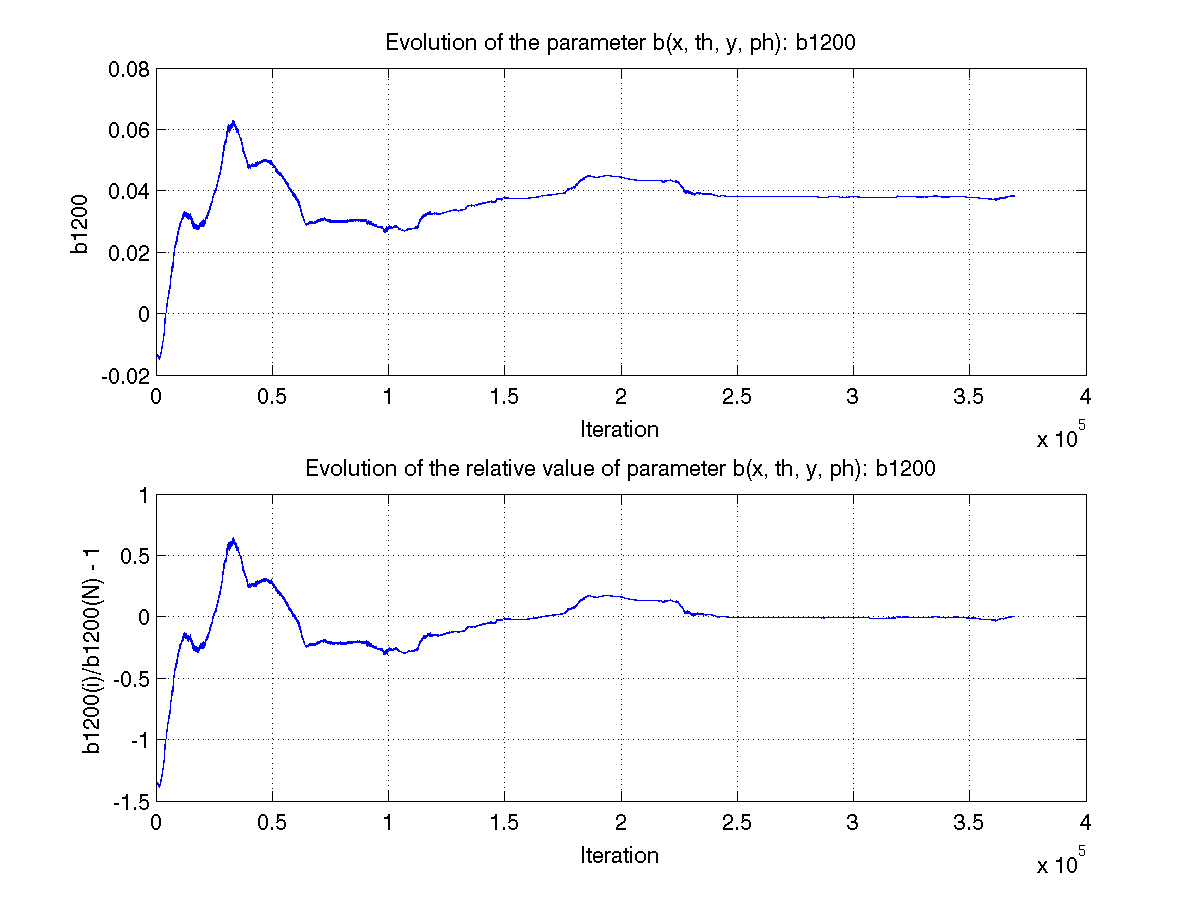
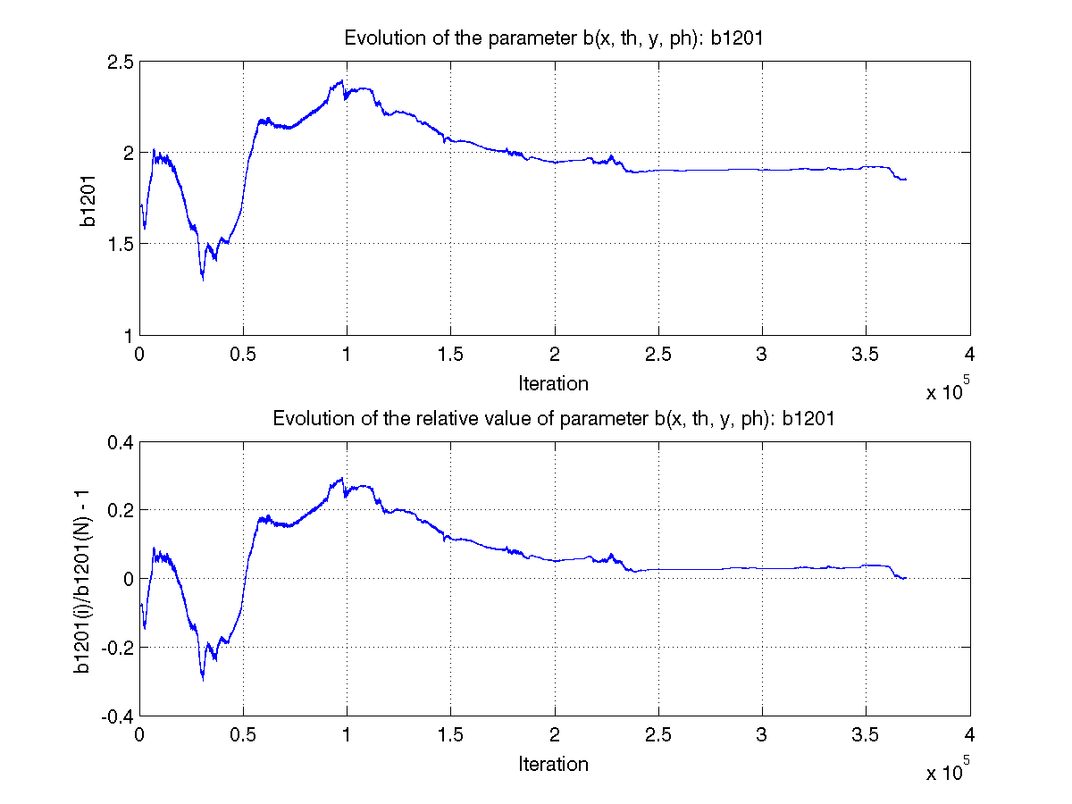
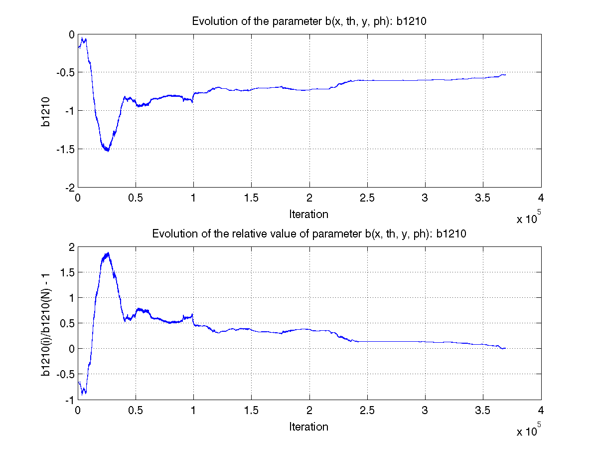
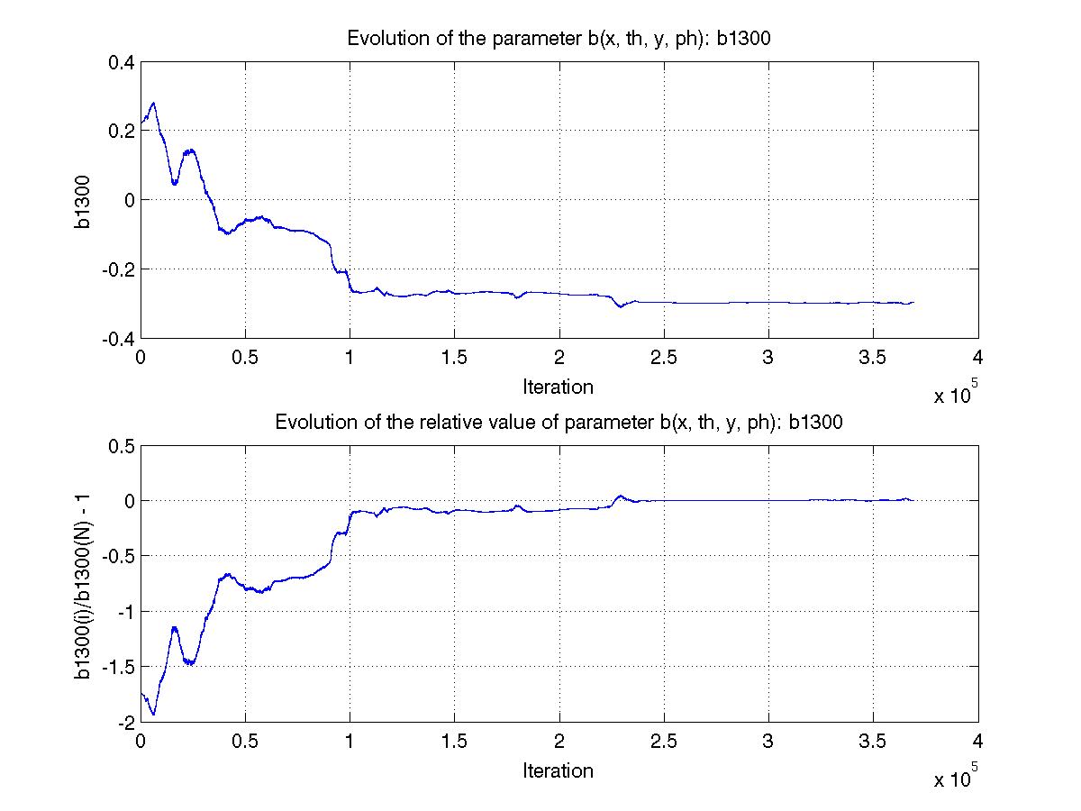
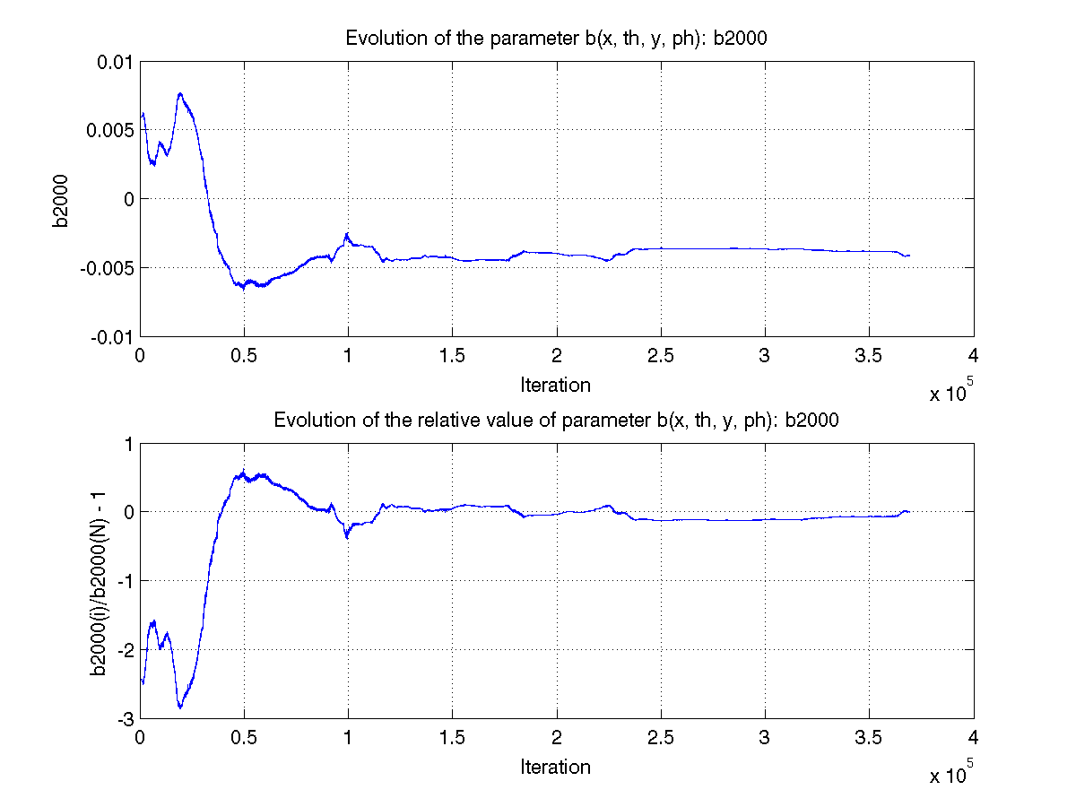
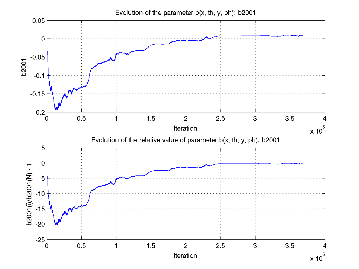
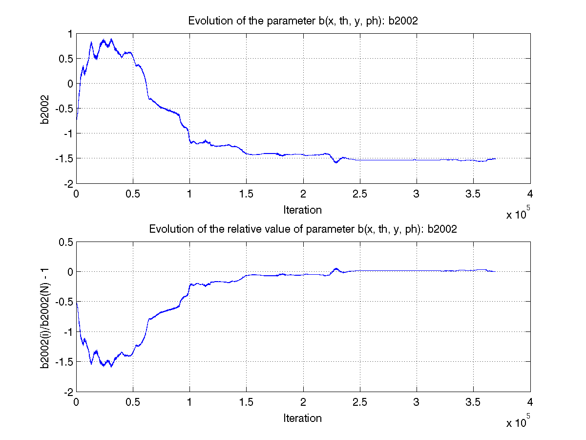
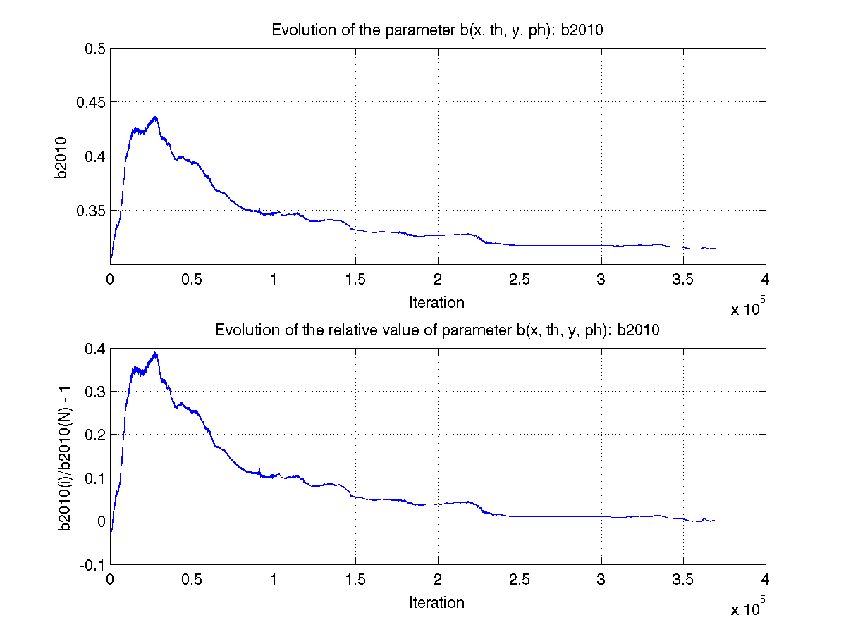
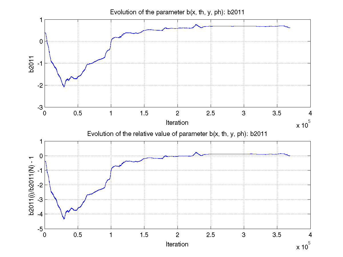
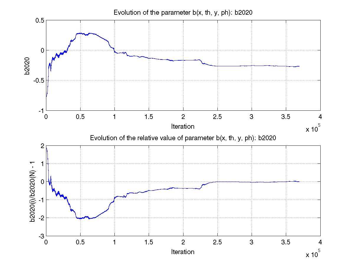
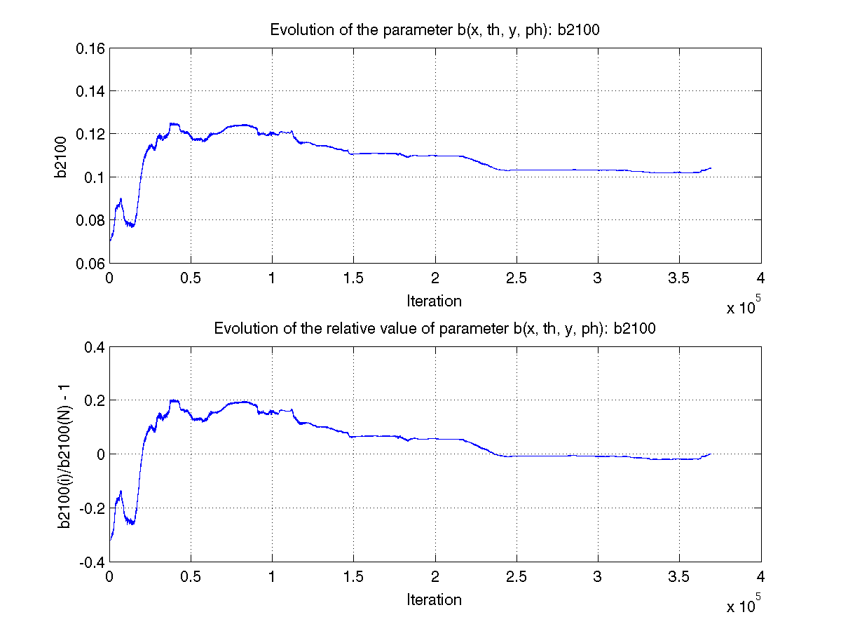
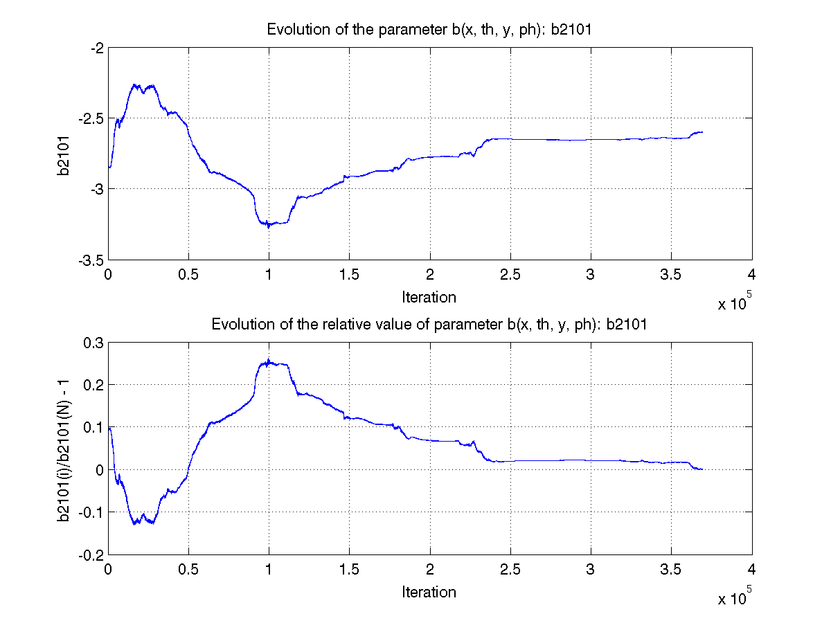
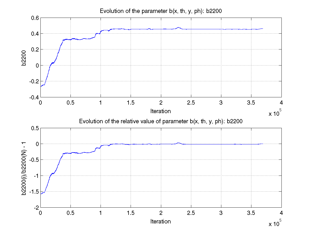
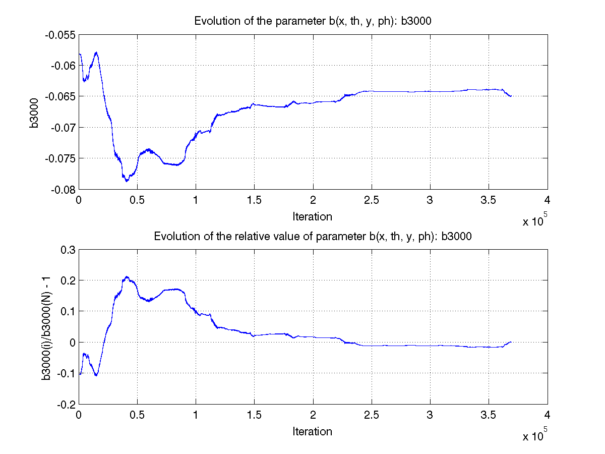
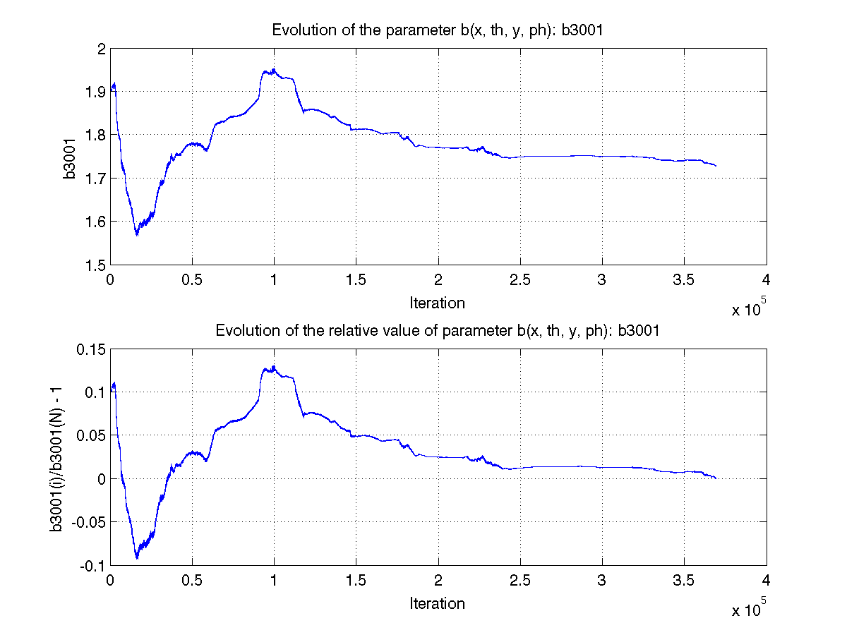
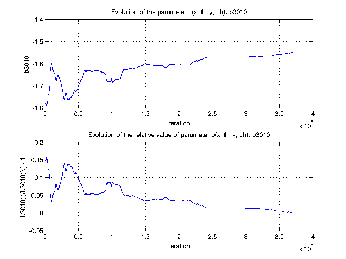
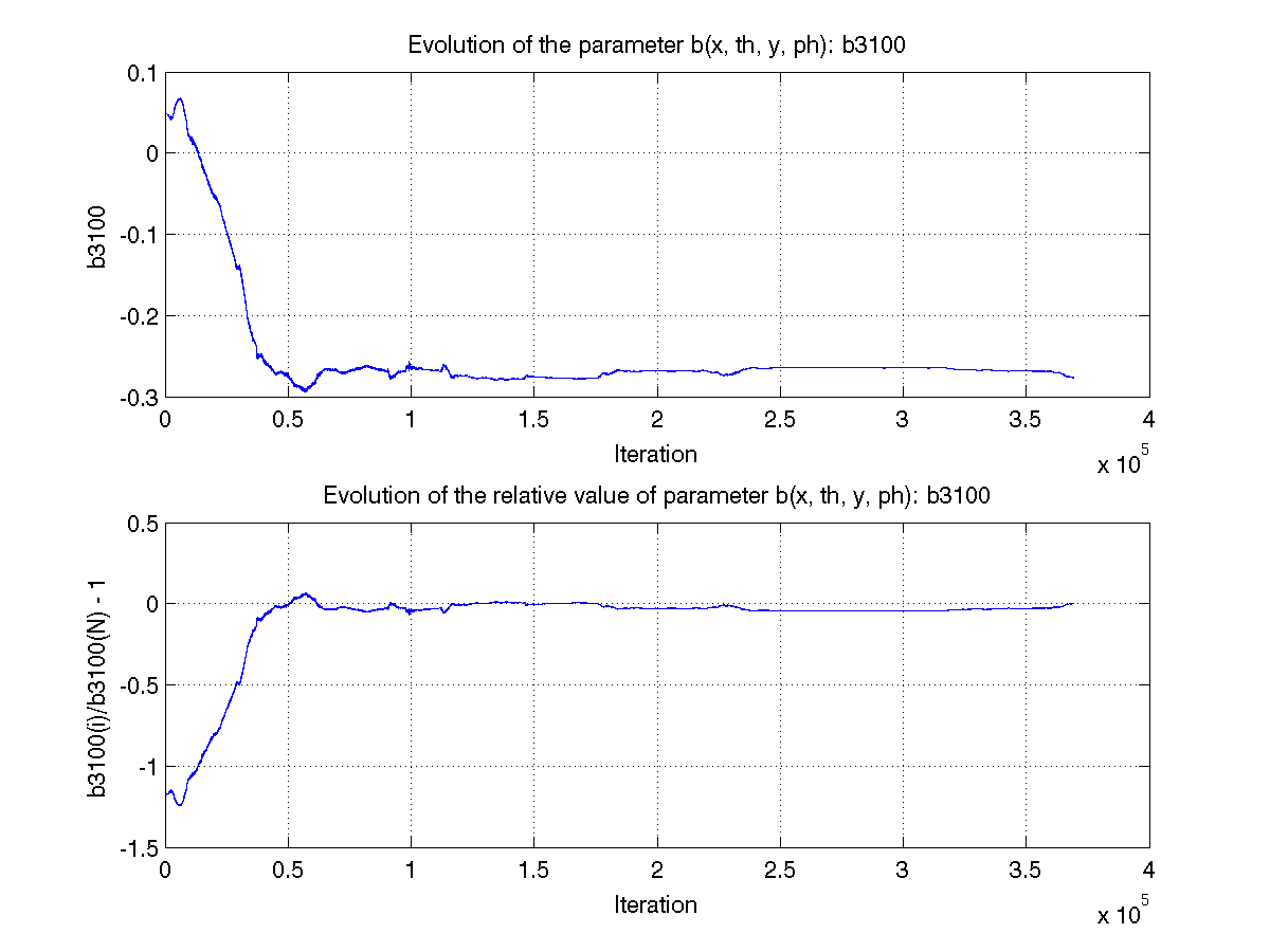
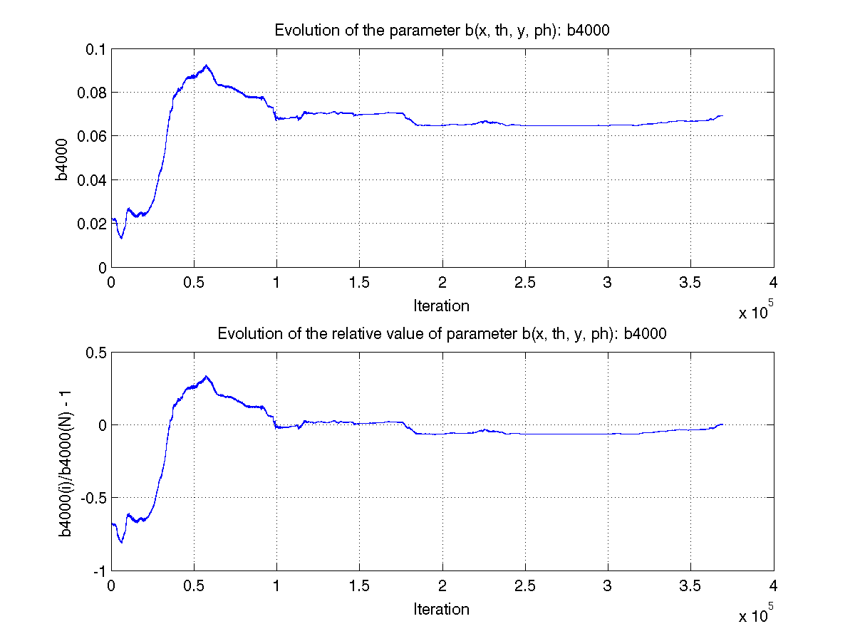
Matrix elements:
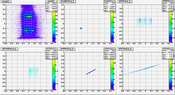
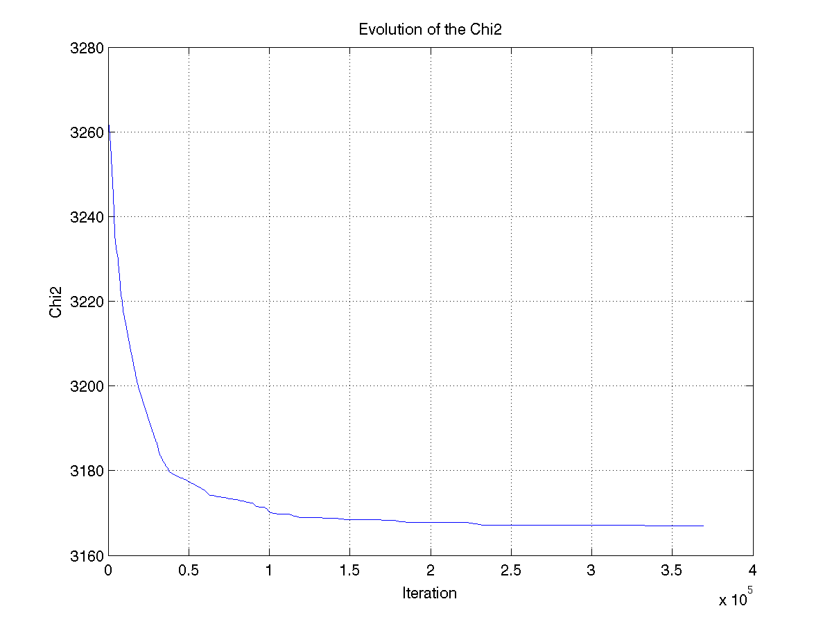
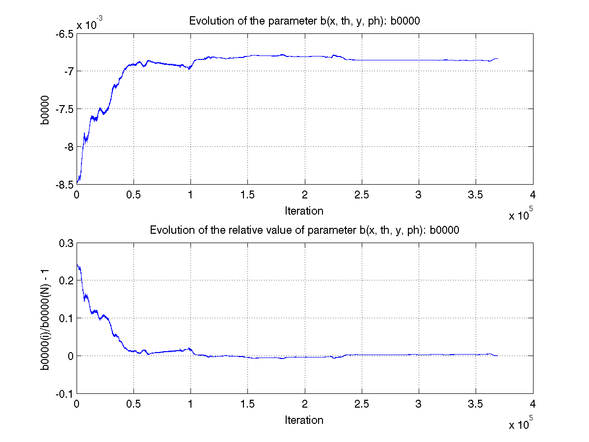
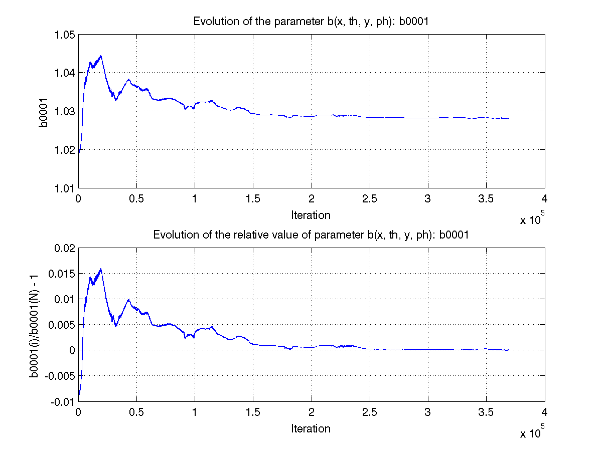
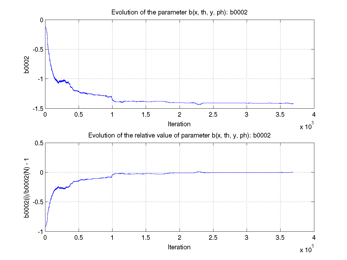
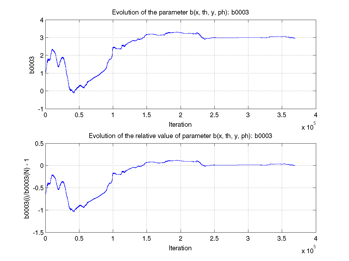
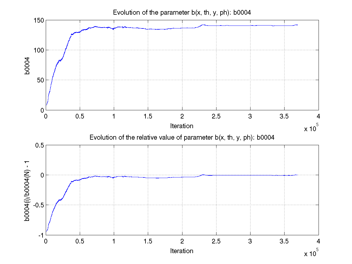
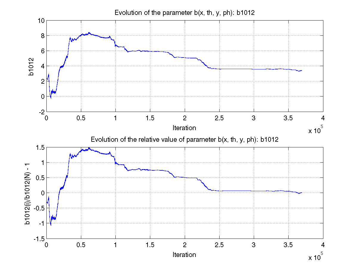
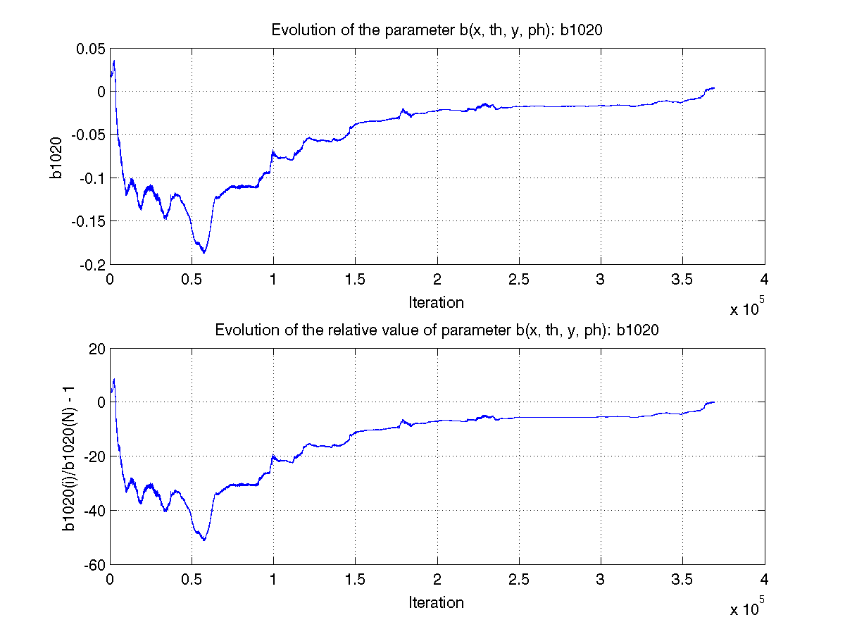
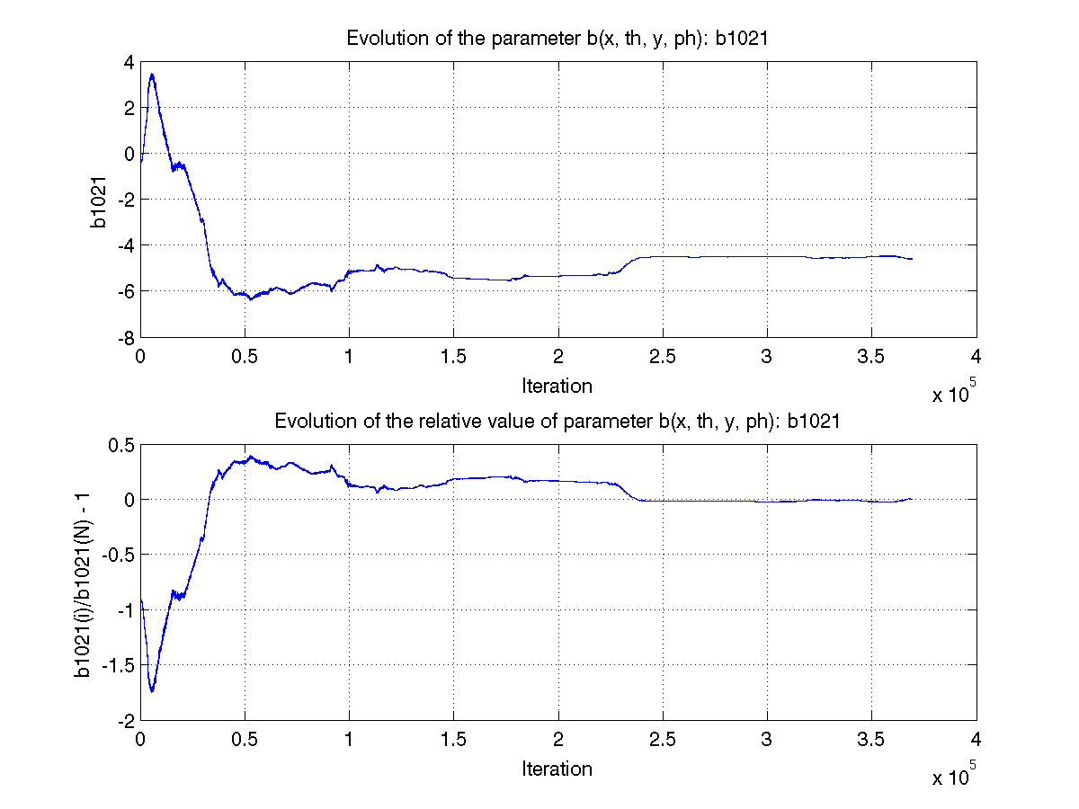
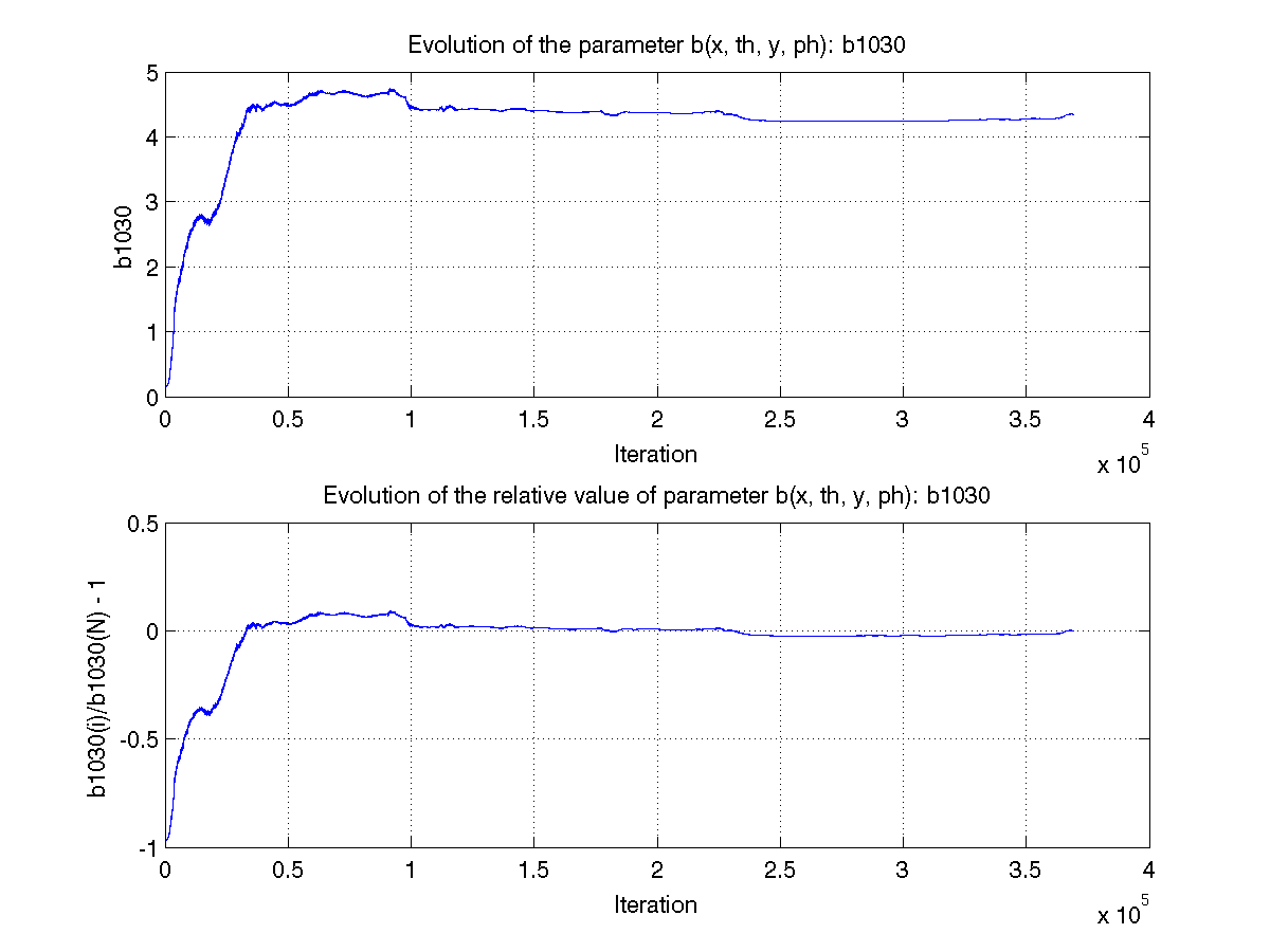
These plots show how various matrix elements change with the number of the iterations made by the
Matlab minimization code:

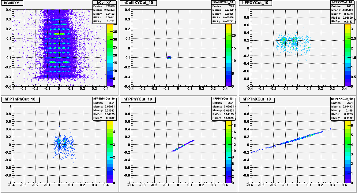
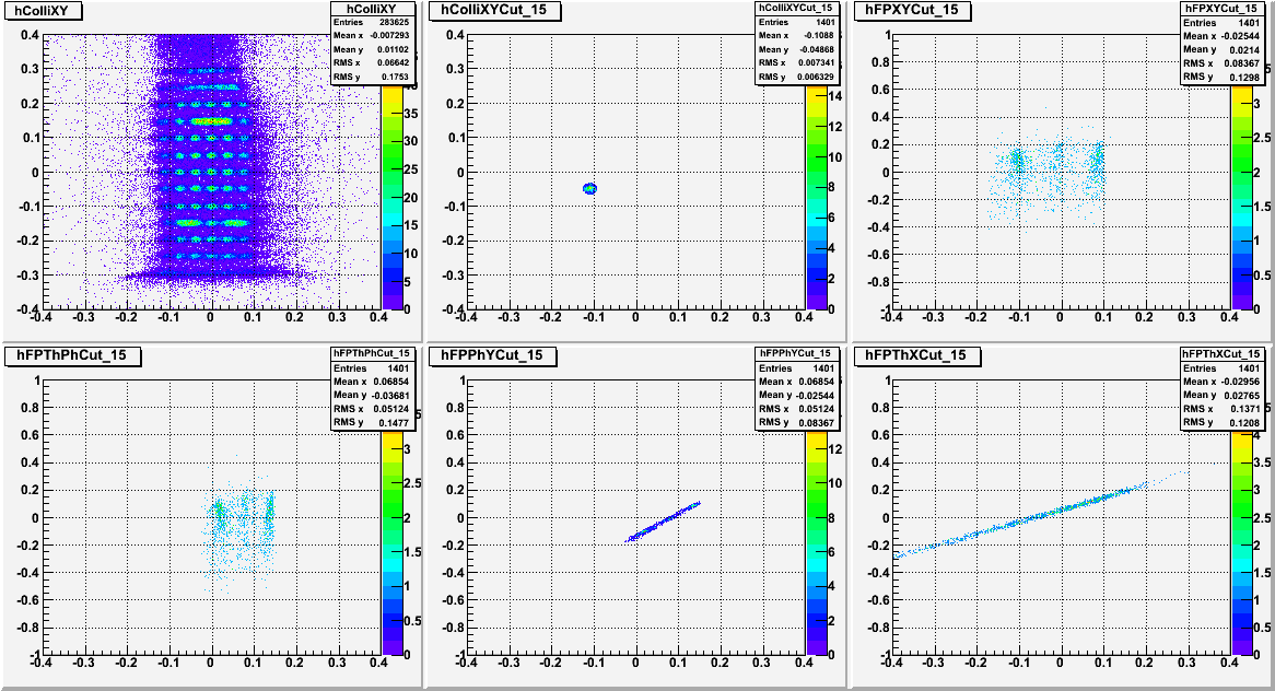
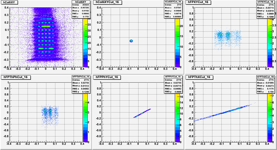
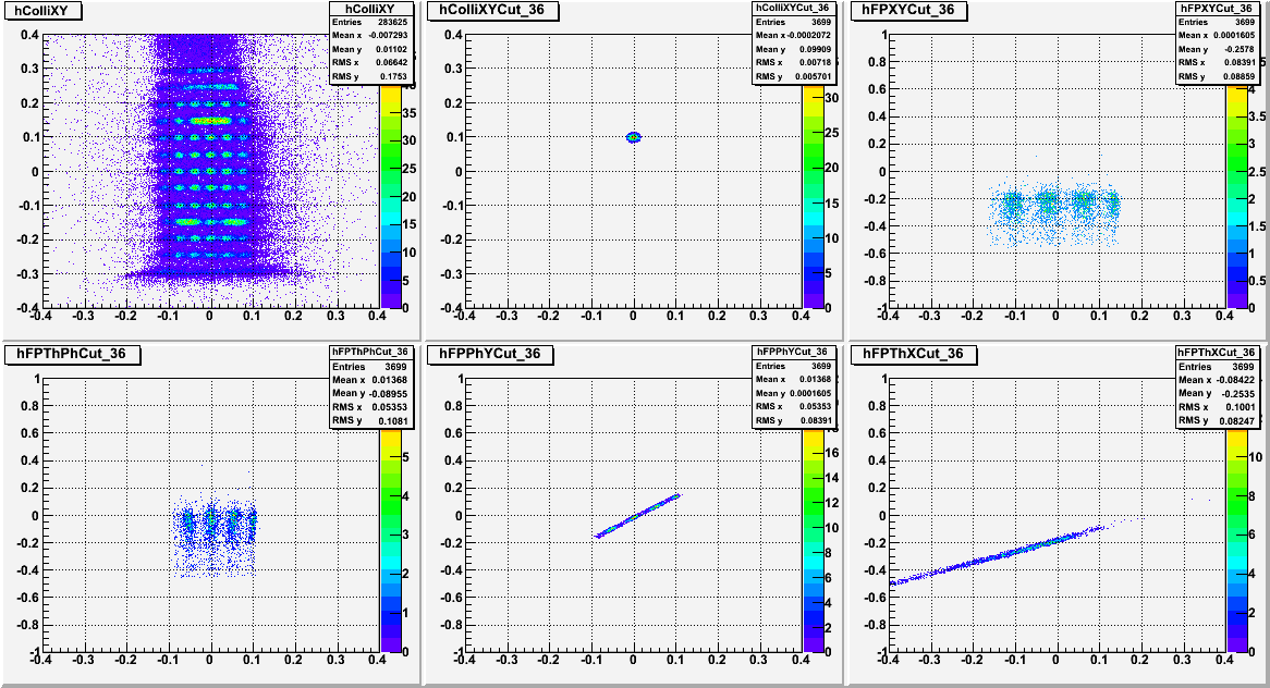
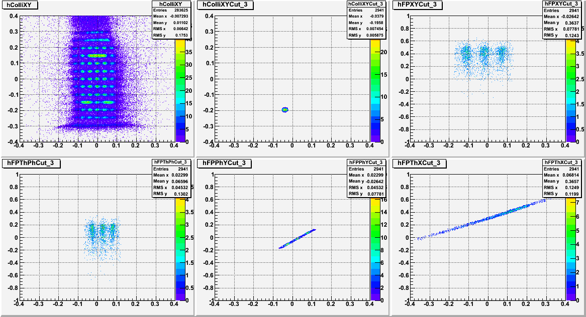
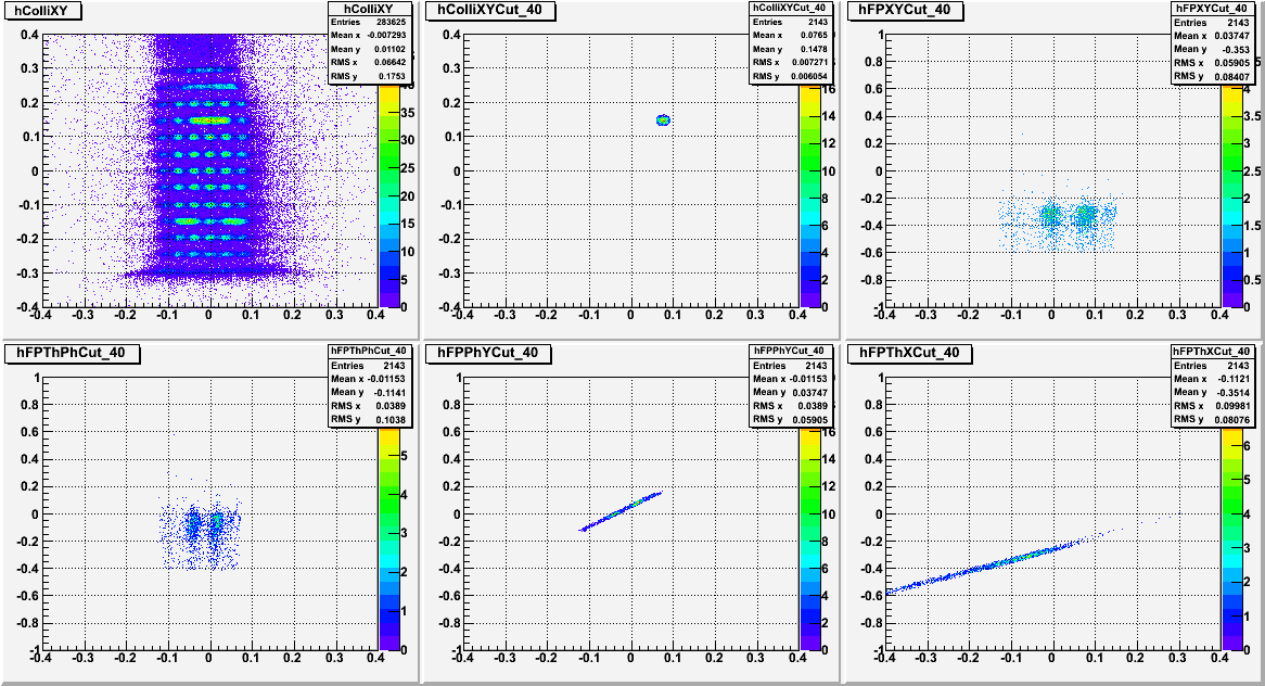
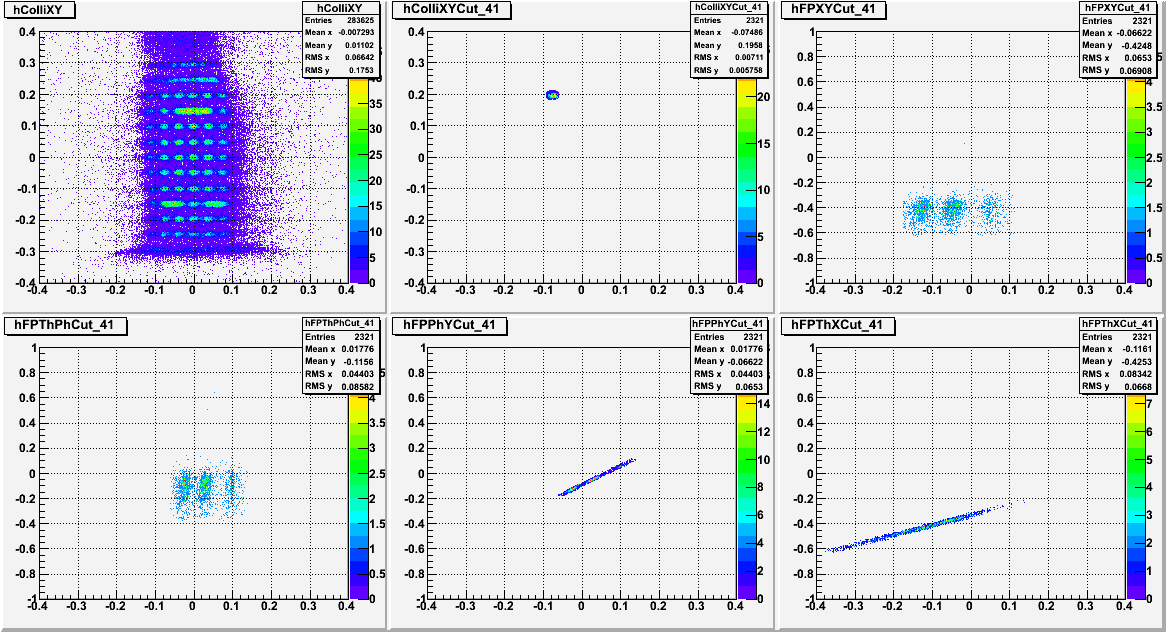
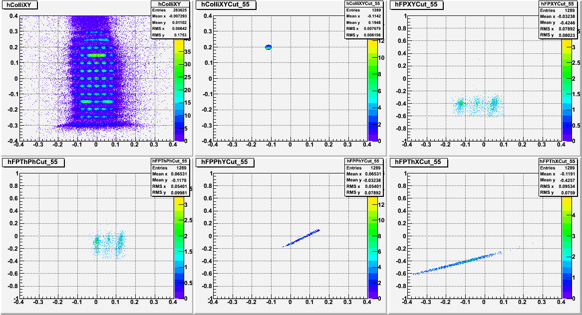
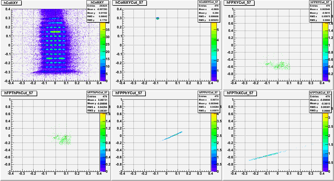
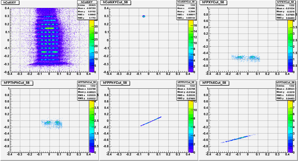
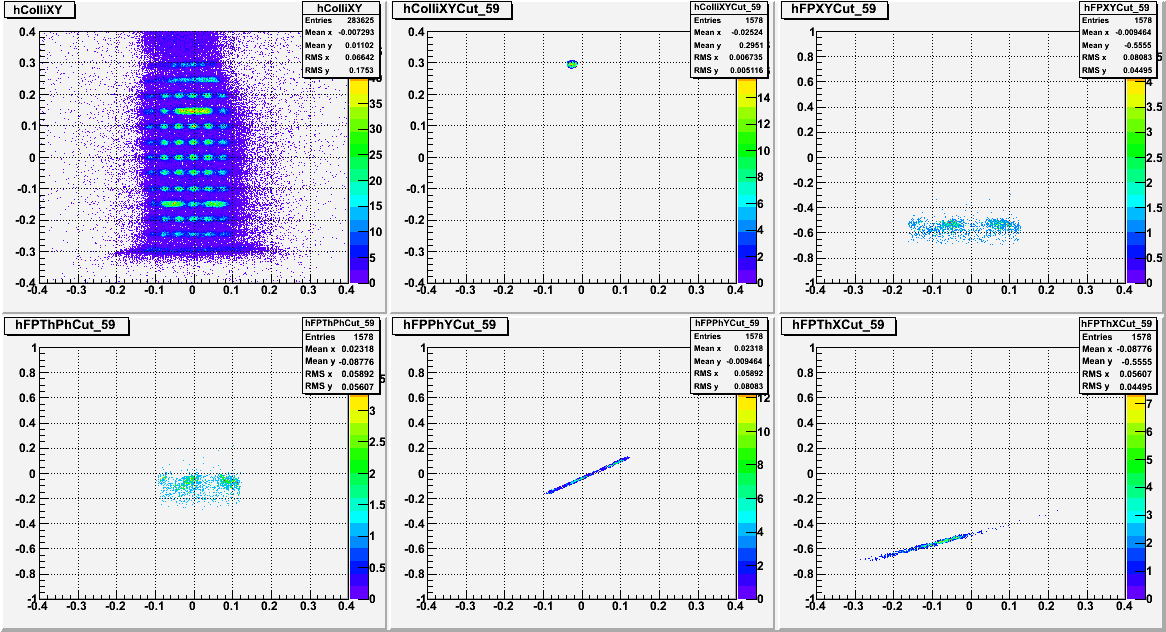
Event selection:
Plots show holes and corresponding events in the focal-plane, that were considered in the matrix
optimization algorithm.


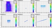
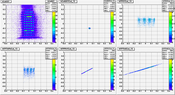

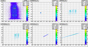
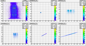
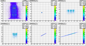

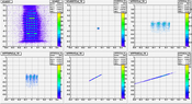

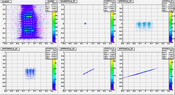
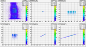
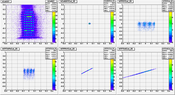
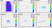
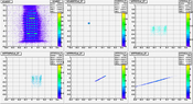
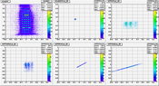
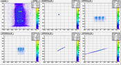

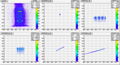
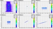

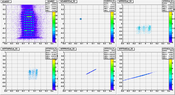


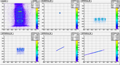

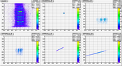
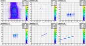
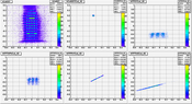
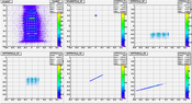
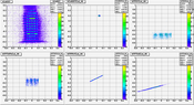

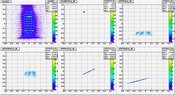

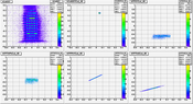

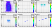
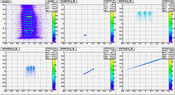
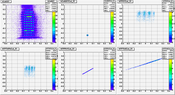
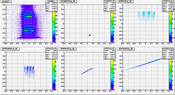

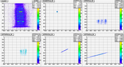

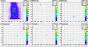
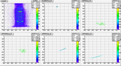
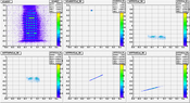
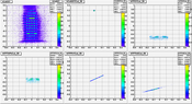

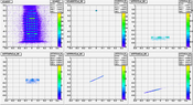

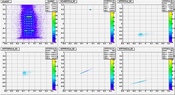
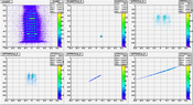


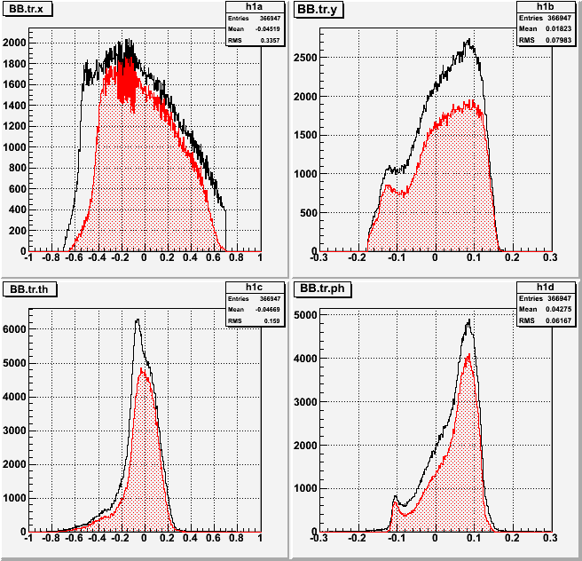
Acceptance ratio:
Plots show the differences in the event-distributions in the focal-plane, caused by the cuts made
in the Sieve-plane:
4.)  5.)
5.)  6.)
6.) 
Last modified: 04/07/10
 4.)
4.) 


 5.)
5.)  6.)
6.)