Optics Calibration - Results:
Here are my currently best results for the BigBite optics calibration. I have determined
matrices for all four target variables TgY, TgTh, TgPh and ThDelta. I have tested various
techniques when trying to determine matrix elements. In the end I have decided to use
SDV (Singular Value Decomposition), which was much faster and more reliable than all other
methods. A nice thing about this method is also that the its solution is by definition the
best one. For methods like stimulated annealing etc. this is not always the case and one must
make sure, that the results returned by such method really represent the global minimum, when
comparing the fitted result with the real ones.
I began the calibration of target variables TgY, TgTh and TgPh with 70 matrix elements (consistent
expansion to fourth order). I used SVD method separately on every available run in order to
determine all 70 matrix elements. Then I compared matrix elements calculated from all analyzed runs
and determined which matrix elements are relevant and which are not. This way I significantly
reduced the number of considered matrix elements in my final matrix.
For the calibration of TgDelta variable I considered slightly different approach. In general
I have two options, when searching for TgDelta matrix. I could determine the TgDelta matrix
elements via missing mass peak calibration. In order to do this I would have to solve non-linear
set of equations. For this I used stimulated annealing method, since SVD can be used only to
solve linear set of equation. I found this method very unstable. The majority of events has
momentum close to central momentum of the BigBite (500MeV/c). Therefore algorithm favors a solution,
where all the matrix elements are close to zero, although they should be non-zero. Therefore I abandoned
this procedure and tried to determine TgDelta matrix elements using the elastic data. This way I had linear
set of equations, because direct comparison of calculated momentum with the q-vector (determined from left arm).
is possible. Therefore I was again able to use SVD to find matrix elements. However, this method has
some limitations:
1.) I have only small number of H,D elastic runs. I addition, these runs do not cover the whole
momentum acceptance of BigBite.
2.) Need to use q.-e. data in combination with simulation to cover the momentum region without elastic data.
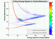
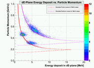
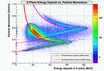
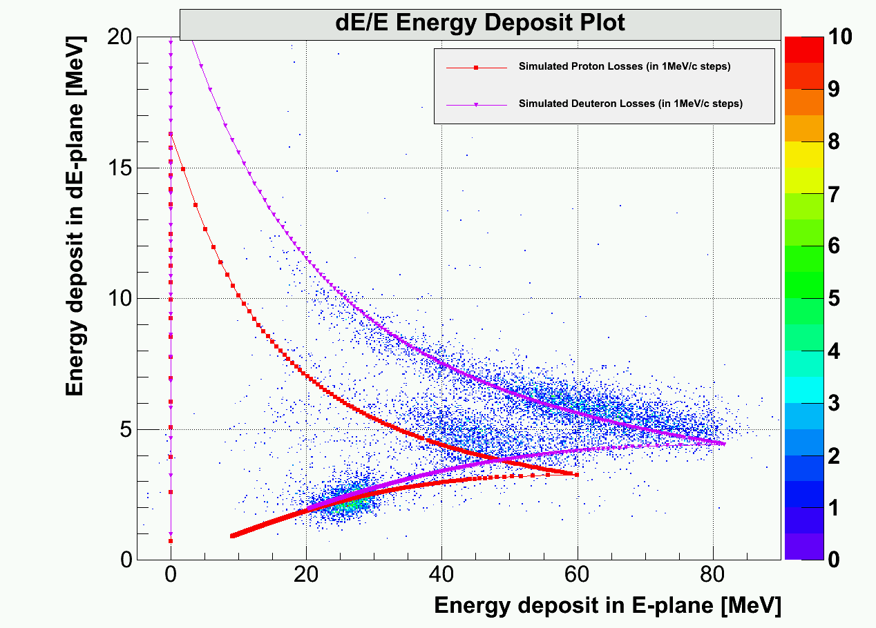
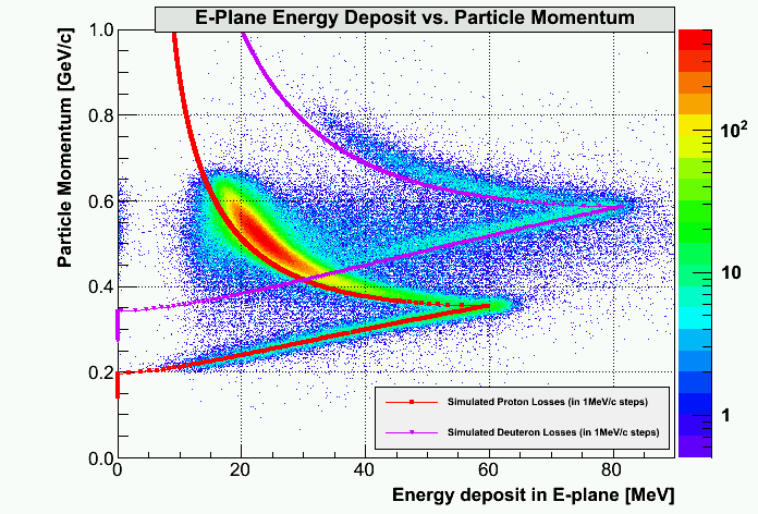
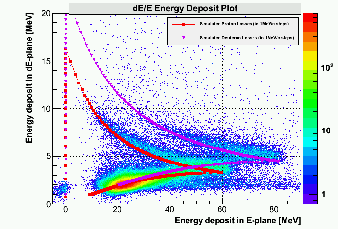
Three well defined points, that I used in my calibration, are the punch-through points for protons and deuterons
in E and dE plane. The particle momentum in each of these points was determined using energy-loss simulation.
At the moment, simulation works with the accuracy to approx. 10MeV/c. The main error comes from not knowing the
correct properties of the materials used in the BigBite and Target system.
3.) In order to form a matrix that workd for deuterons as well as for protons, a BigBite momentum ie.
TgDelta must not be directly compared to the q-vector, but must be properly corrected for energy-losses.
I determined, that this way matrix works much better than without correction.
4.) Since all the events in an elastic runs are at the fixed in-plane angle ie. single value of FpY and FpPh, I
could consider only FpTh and FpX dependence on TgDelta. In spite of this limitation, the matrix seems to be working
quite well.
The Matrix
[matrix]
t 1 0 0  0.0000E+00  0.0000E+00  0.0000E+00  0.0000E+00  0.0000E+00  0.0000E+00   0.0000E+00
y 1 0 0  0.0000E+00  0.0000E+00  0.0000E+00  0.0000E+00  0.0000E+00  0.0000E+00   0.0000E+00
p 1 0 0  0.0000E+00  0.0000E+00  0.0000E+00  0.0000E+00  0.0000E+00  0.0000E+00   0.0000E+00

D 0 0 0  -0.08749  -0.67627   1.91361  -3.11562  -6.33754   11.5908
D 1 0 0   2.80163  -8.35861   17.7113   17.3145  -56.5428   0.00000
D 2 0 0   11.6524  -46.0247   7.91907   119.282   0.00000   0.00000
D 3 0 0   44.3530  -77.9449  -99.1704   0.00000   0.00000   0.00000
D 4 0 0   79.0134  -4.96614   0.00000   0.00000   0.00000   0.00000
D 5 0 0   42.3238   0.00000   0.00000   0.00000   0.00000   0.00000
D 0 0 0   0.00000   0.00000   0.00000   0.00000   0.00000   0.00000

T 0 0 0   0.01628   0.52262  -0.05985  -0.05323   0.07144
T 0 0 1   0.00000  -0.24186   0.00000   0.00139   0.00000
T 0 0 2  -0.01478   0.03324   0.00000   0.00000   0.00000
T 0 0 3   0.00000   2.27640   0.00000   0.00000   0.00000
T 0 1 0   0.00000   0.08945   0.00000   0.00000   0.00000
T 0 1 1   0.00000  -0.08372   0.00000   0.00000   0.00000
T 0 1 2   0.00000  -4.22919   0.00000   0.00000   0.00000
T 0 2 0   0.00000   0.08359   0.00000   0.00000   0.00000
T 0 2 1   0.00000   1.83541   0.00000   0.00000   0.00000
T 1 0 0  -0.45961  -0.02880   0.09455  -0.08116   0.00000
T 1 0 1   0.28138   0.00000   0.11322   0.00000   0.00000
T 1 0 3  -3.08268   0.00000   0.00000   0.00000   0.00000
T 1 1 0  -0.08642   0.00000   0.00000   0.00000   0.00000
T 2 0 0   0.04289   0.00000  -0.02958   0.00000   0.00000
T 2 0 1   0.00000  -0.54018   0.00000   0.00000   0.00000

P 0 0 0   0.00873   0.00654   0.00433  -0.03137  -0.05554
P 0 0 1   1.00197  -0.22111   0.00000   0.00000   0.00000
P 0 0 2  -1.85838  -1.08076   0.00000   0.00000   0.00000
P 0 0 3   24.2962   2.50163   0.00000   0.00000   0.00000
P 0 1 0  -0.01622   0.10266   0.09110  -1.17133   0.00000
P 0 1 1   2.34751   1.09849   0.00000   0.00000   0.00000
P 0 1 2  -35.4271   0.00000   0.00000   0.00000   0.00000
P 0 1 3  -21.9948   0.00000   0.00000   0.00000   0.00000
P 0 2 0  -0.87079   0.00000   0.00000   0.00000   0.00000
P 0 2 1   22.0197   0.00000   0.00000   0.00000   0.00000
P 0 3 0  -5.43382   0.00000   0.00000   0.00000   0.00000
P 0 3 1   10.3034   0.00000   0.00000   0.00000   0.00000
P 1 0 0   0.00000   0.01358   0.04407   0.10015   0.00000
P 1 0 1   0.00000   0.00000   1.13845   0.00000   0.00000
P 1 0 3   4.33170   0.00000   0.00000   0.00000   0.00000
P 1 1 0   0.12449  -0.07625   1.29633   0.00000   0.00000
P 1 1 1   0.83016  -0.37522   0.00000   0.00000   0.00000
P 1 2 0  -0.73711   0.00000   0.00000   0.00000   0.00000
P 1 2 1  -5.73354   0.00000   0.00000   0.00000   0.00000
P 2 0 0   0.00000   0.00167  -0.02580   0.00000   0.00000
P 2 0 1   0.00000  -1.15315   0.00000   0.00000   0.00000
P 2 1 0   0.46776  -0.07927   0.00000   0.00000   0.00000

Y 0 0 0   0.02420   0.00000
Y 0 0 1  -2.77260   0.00000
Y 0 0 2  -1.33277   0.97479
Y 0 0 3  -15.1454   0.00000
Y 0 0 4   212.594   0.00000
Y 0 1 0   1.00077  -0.11737
Y 0 1 1   0.81629  -1.51468
Y 0 1 2   7.43661   0.00000
Y 0 1 3  -251.699   0.00000
Y 0 2 0   0.00000   0.35839
Y 0 2 2   107.362   0.00000
Y 0 3 1  -22.7024   0.00000
Y 1 0 0   0.00496   0.00000
Y 1 0 2   0.35765   0.00000
Y 1 1 0   0.18844   0.00000
Y 1 1 1  -0.27074   0.00000
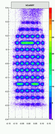
Results for Carbon Optics runs:
1.)  2.)
2.) 
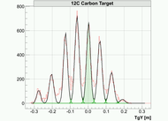
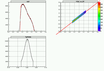
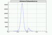
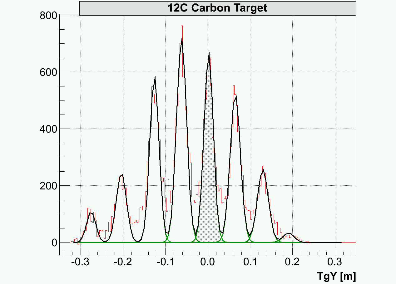
Plots show results for TgY calibration, using 7-foil carbon target. The best resolution for TgY, that I could get is \sigma_{TgY} = 1.1cm. When using gaseous targets, the resolution worsens and gets
closer to \sigma_{TgY} \approx 2cm.
Results for Carbon Optics runs with sieve-in:
3.) 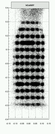 4.)
4.) 
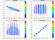
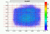
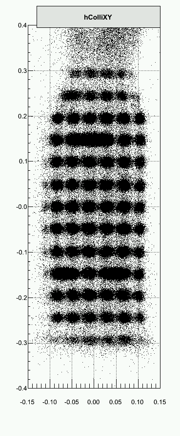
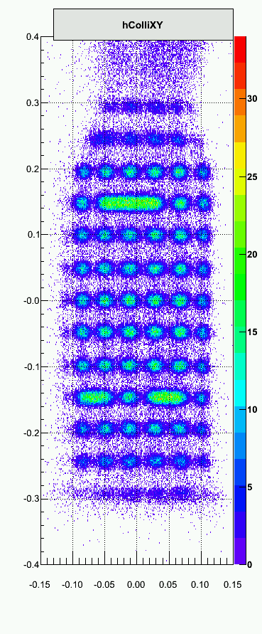
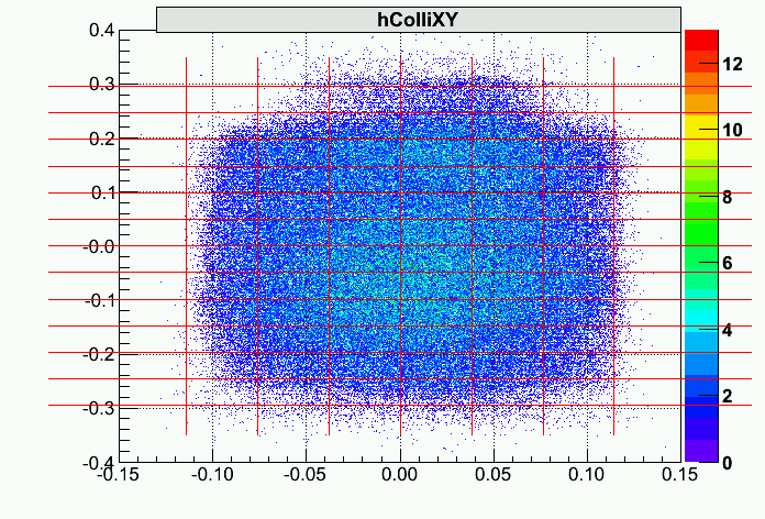
Plots show the reconstructed BigBite sieve pattern. We can see the majority of holes. Holes on the left side of BigBite are not visible, because they are outside the BigBite acceptace. For the same reason some of the
holes on the edges of the sieve slit are also missing .
Results for Elastic H,D runs:
5.)  6.)
6.)  7.)
7.)  8.)
8.) 
9.)  10.)
10.)  11.)
11.) 
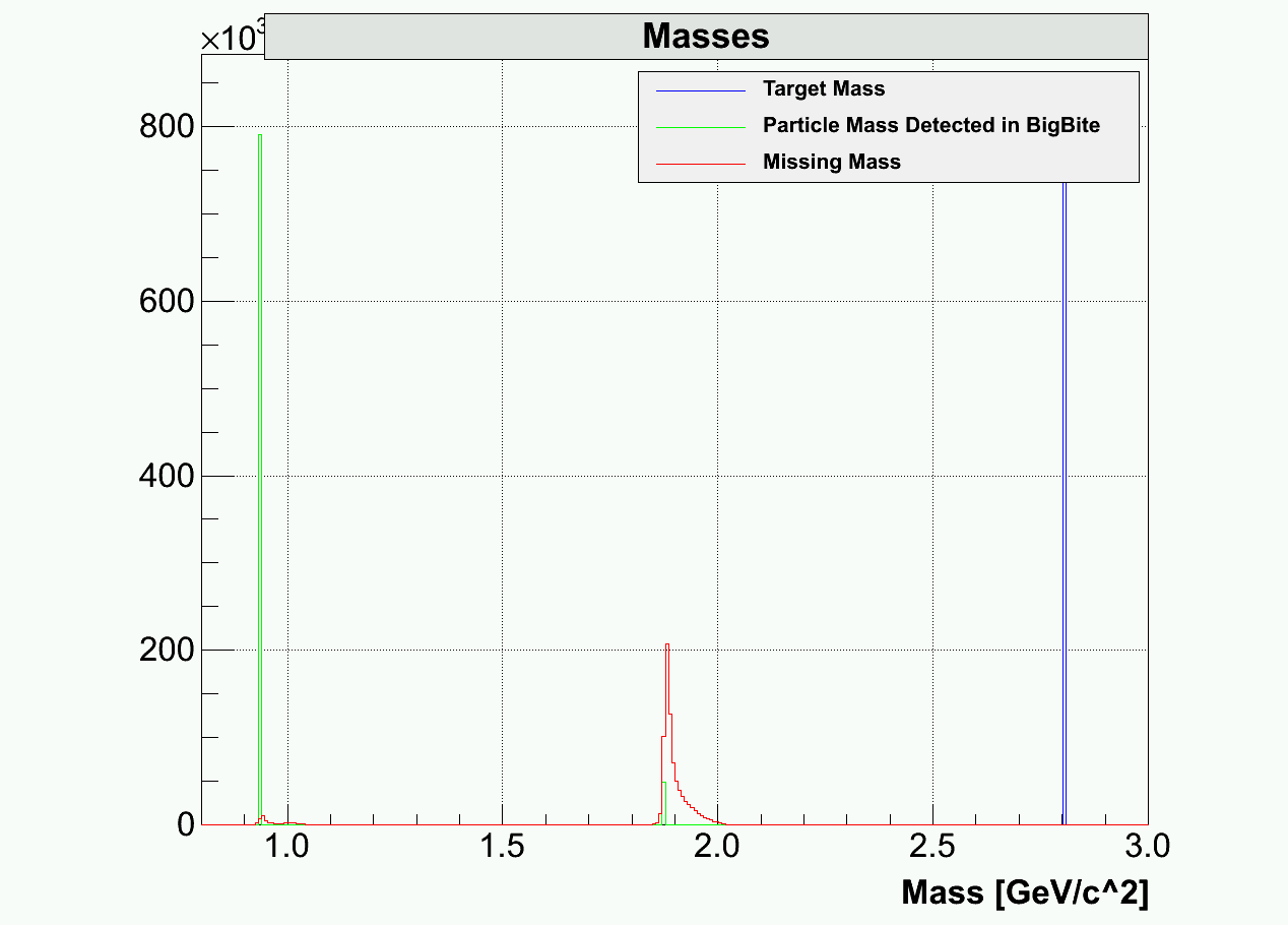
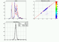
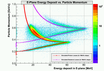
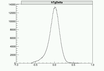
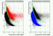
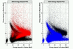
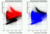
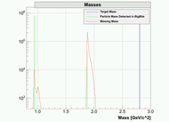
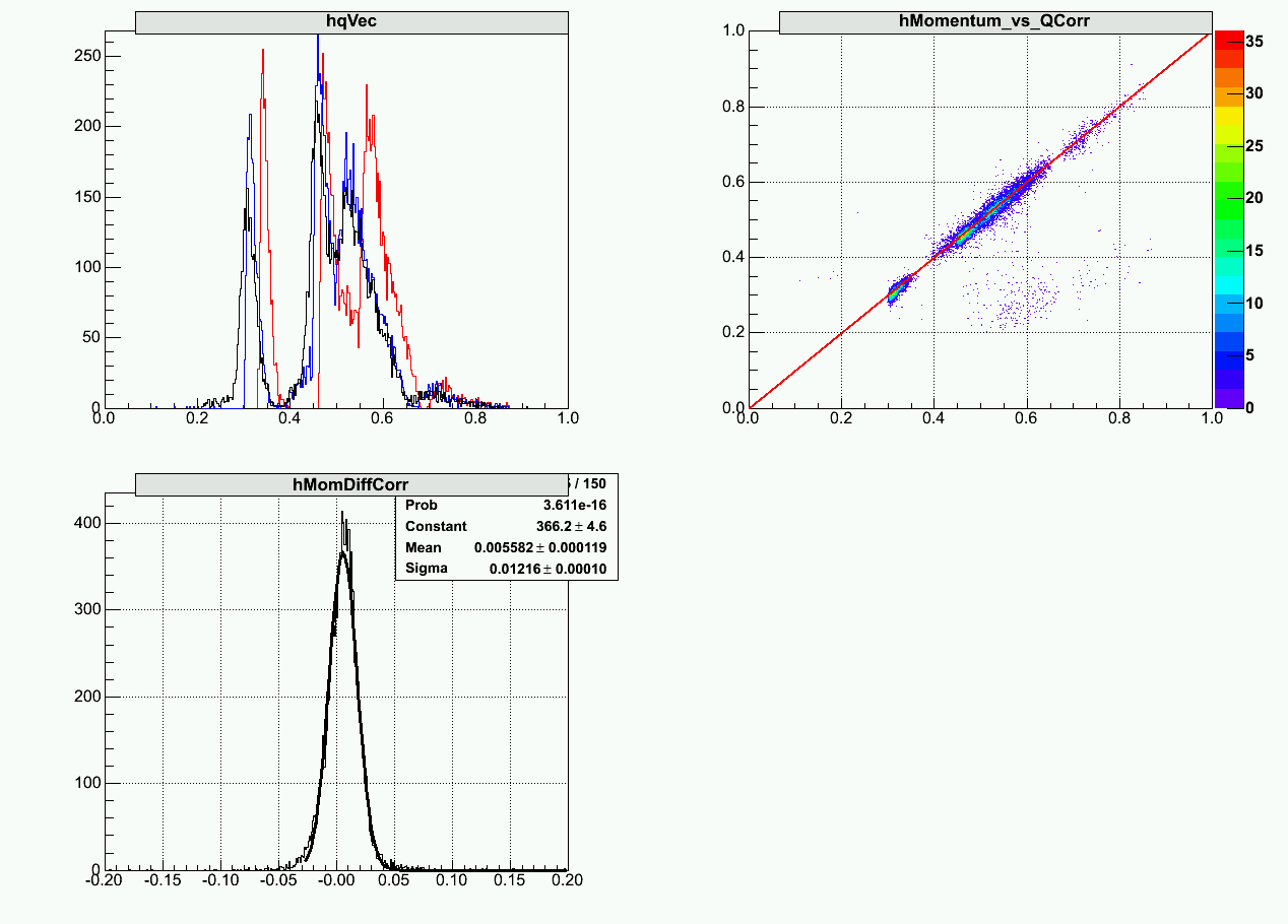
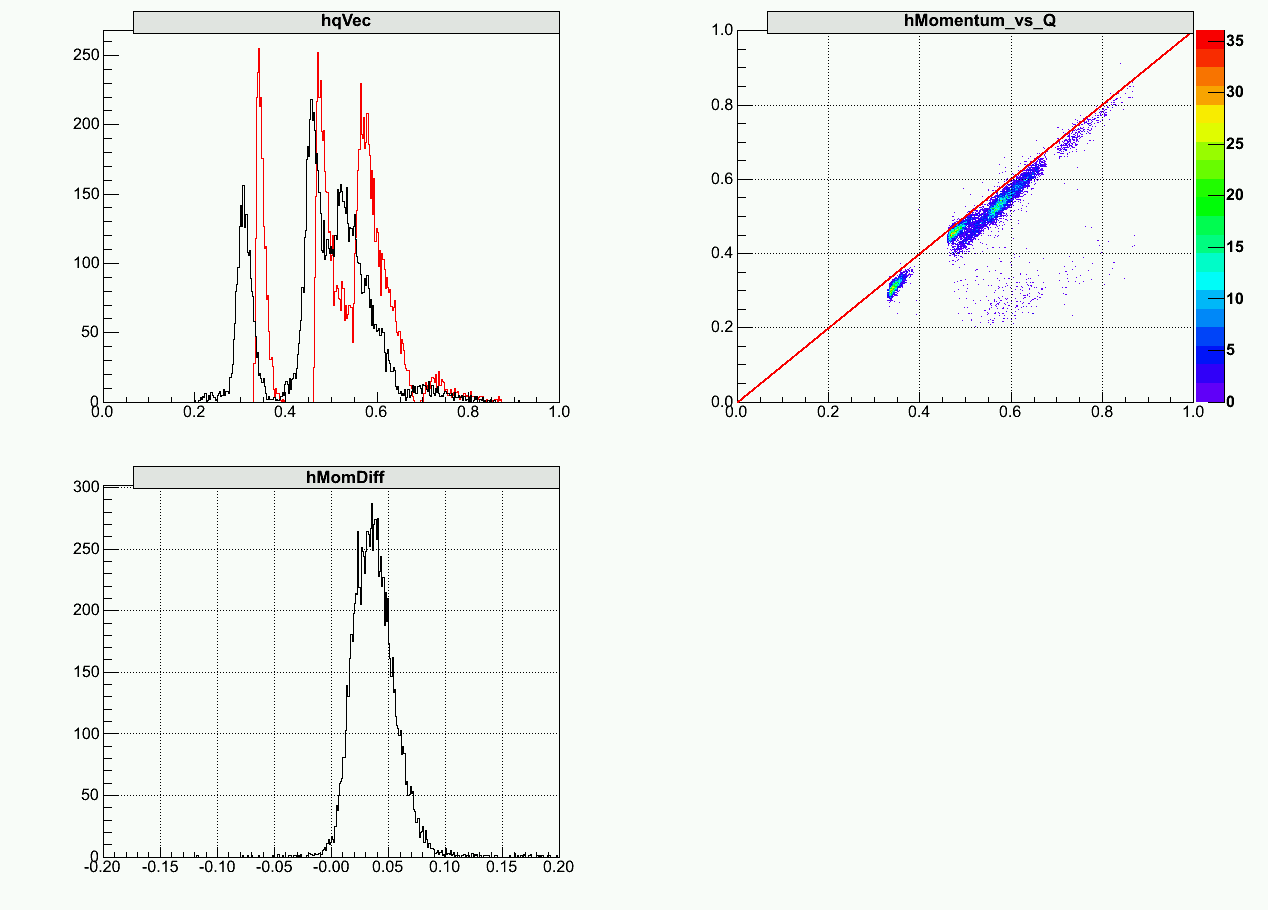
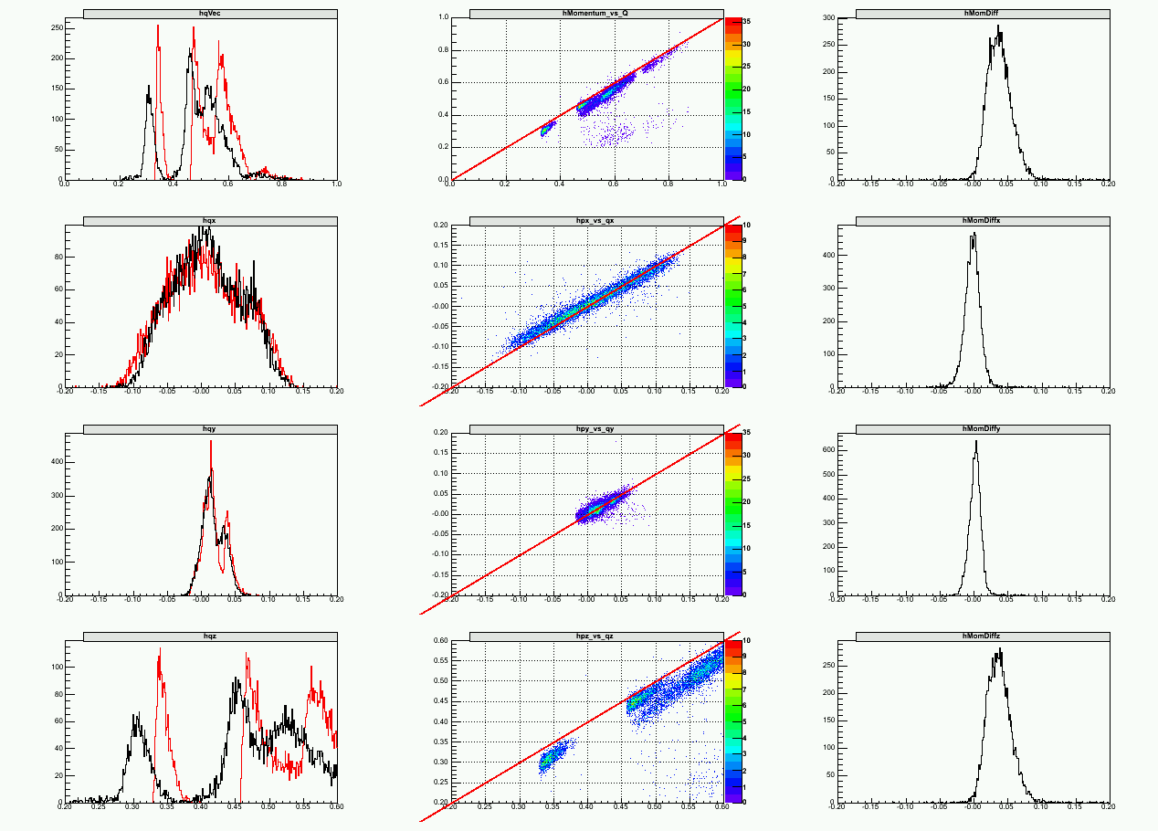
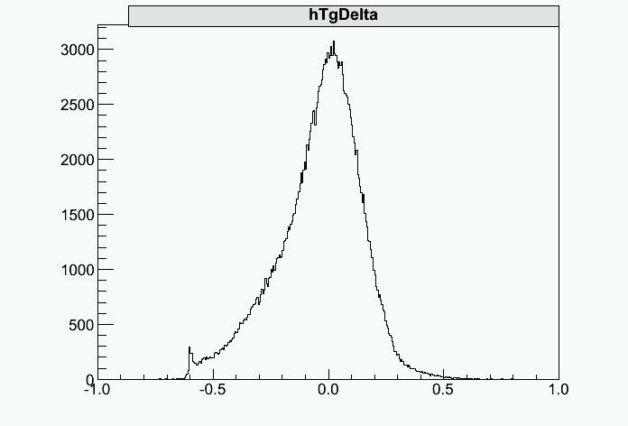
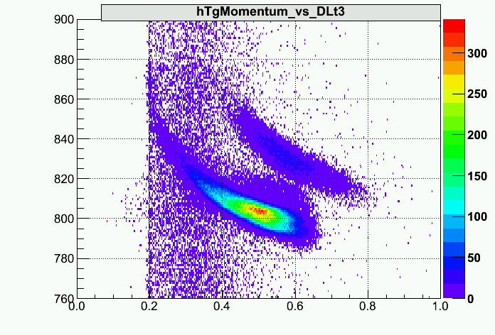
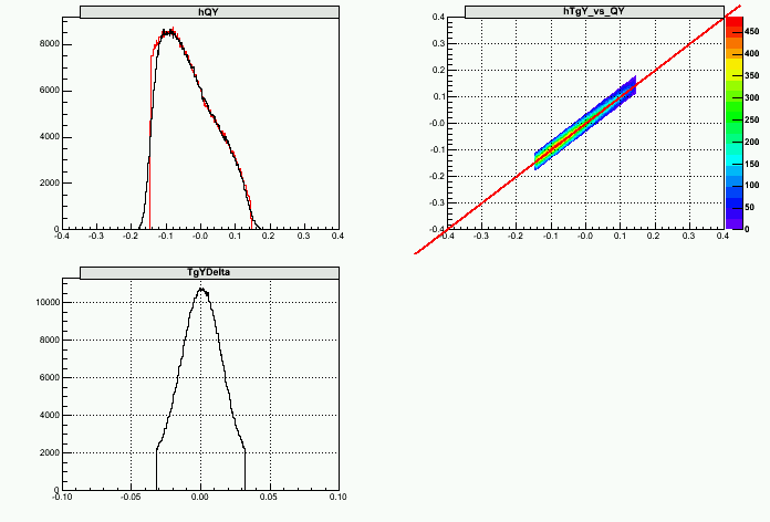
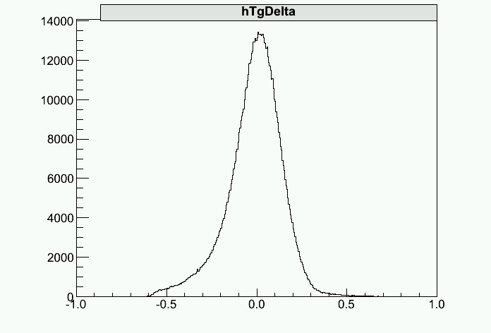
Plot 5.) shows results for TgDelta calibration. They display the comparison of reconstructed BB momentum versus the q-vector, corrected for the energy-losses. Plots show all available elastic data available: 2GeV, 3GeV elastic Deuteron data and 1GeV, 2GeV proton data. In the calibration I considered only elastic D data, because they cover bigger portion of BigBite acceptance. Hydrogen data on the other hand, were used only to test the quality of my calibration. From the results you can see, that there is still a small difference Delta_{TgP} \approx 6MeV/c between q-vector and BigBite momentum. I believe, that it comes from the fact, that I do not understand energy losses completely. I apready stated in the beginning that my energy-loss estimator works with the precision to approx 10MeV/c. The estimated resolution of the BigBite momentum reconstruction is \sigma_{Tg_Momentum} \approx 12MeV/c which is approximately 2.5%.
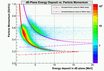
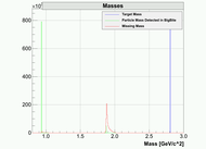
From plot 6.) you can see, that the offset in momentum as well as the width of the distribution is much bigger if the energy-losses are not taken properly into account and q-vector is directly compared to BB momentum.
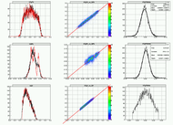
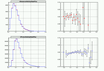
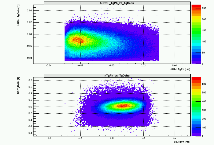
Plot 8.) show the calibration results for TgTh and TgPh. The resolution for TgPh is \sigma_{TgPh} = 1.7E-2, while the resolution in TgTh is \sigma_{TgTh} = 1.9E-2.
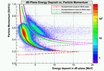
Considered Energy Losses:
12.) 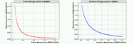
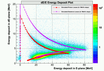
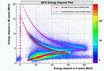
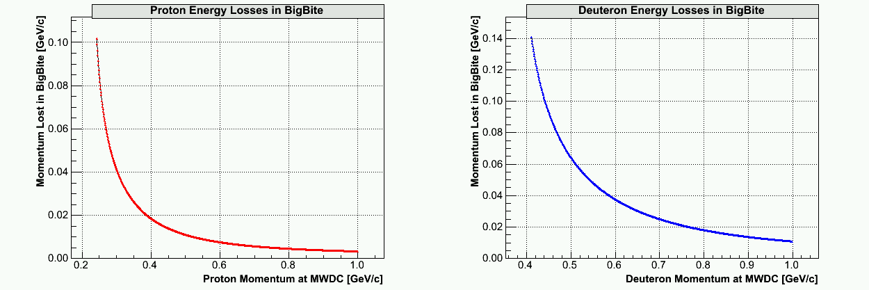
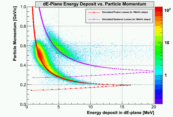
Plot shows particle momentum lost in BigBite spectrometer as a function of the particle momentum at the MWDCs. These energy losses for eacy particle must be then added to reconstructed BB momentum in order to fully reconstruct q-vector.
Results for Production Runs:
13.)  14.)
14.)  15.)
15.)  16.)
16.)  17.)
17.)  18.)
18.) 
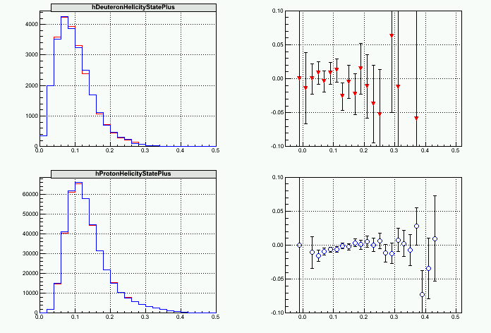
Here are some of the results for production runs on polarized 3He target.
Quick Analysis results:
I have begun working on production data analysis. I am writing a script that will calculate asymmetries.
Here are some preliminary results:
19.)  20.)
20.)  21.)
21.) 
22.)  23.)
23.)  24.)
24.) 
25.)  26.)
26.)  27.)
27.)  28.)
28.) 
29.)  30.)
30.) 
31.) 
Last modified: 01/05/11

 4.)
4.) 
 6.)
6.)  7.)
7.)  8.)
8.) 
 10.)
10.)  11.)
11.) 
 14.)
14.)  15.)
15.)  16.)
16.)  17.)
17.)  18.)
18.) 
 20.)
20.)  21.)
21.) 
 23.)
23.)  24.)
24.) 
 26.)
26.)  27.)
27.)  28.)
28.) 
 30.)
30.)