Photon Energy Correction in EC Using method discribed in CLAS NOTE 2006-015 PASS2
1. Why correct photons?
Pi0 invariant mass is off its 0.135 GeV value by:
C: ~0% and +4.8%(for z>0.4)
Fe: -3.7% and +1.2%(for z>0.4)
Pb: ~0% and +4.2%(for z>0.4)
D has the same Pi0 mass offset as accompanying solid target

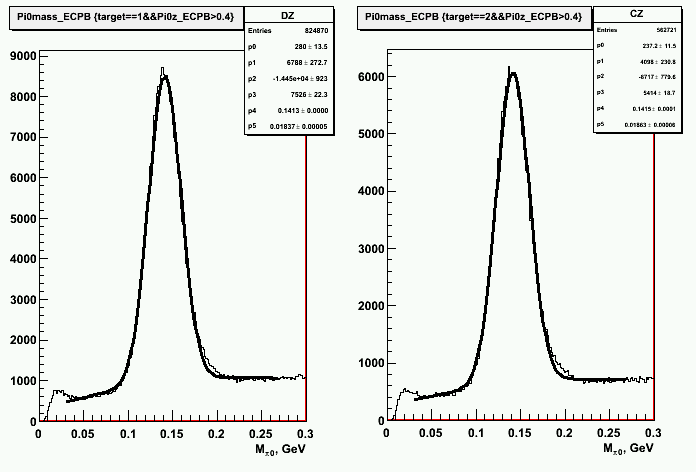
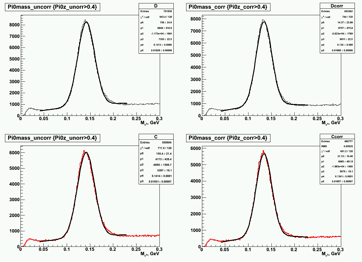
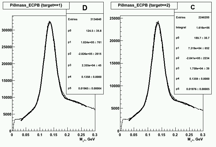
Pi0 invariant mass for Carbon and its D. Left two plots are all Pi0, right are with Z>0.4:
/>

R e s u l t.
Correction for C, Pb (+D):
1.129-0.05793/E-1.0773e-12/(E*E)


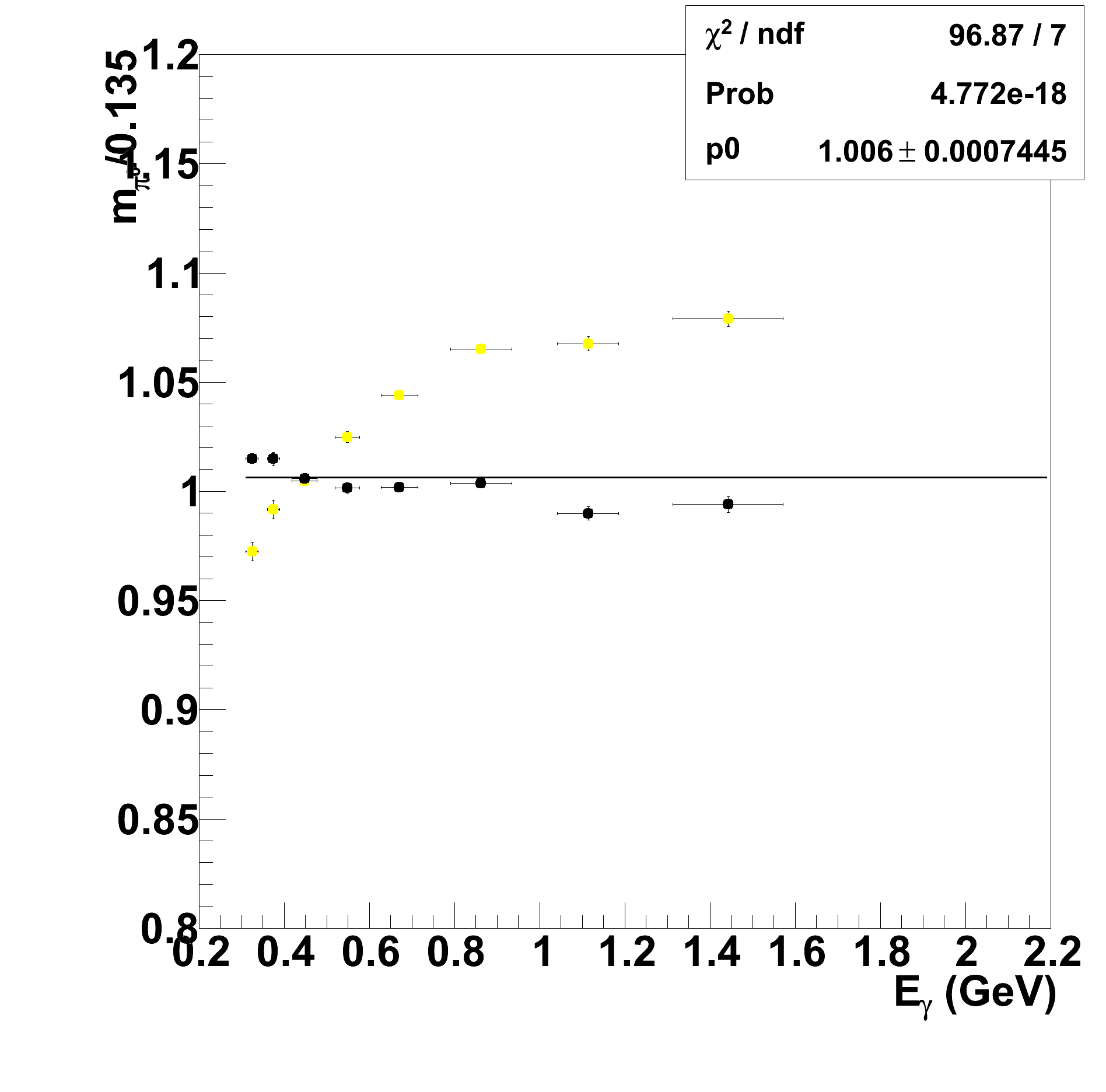
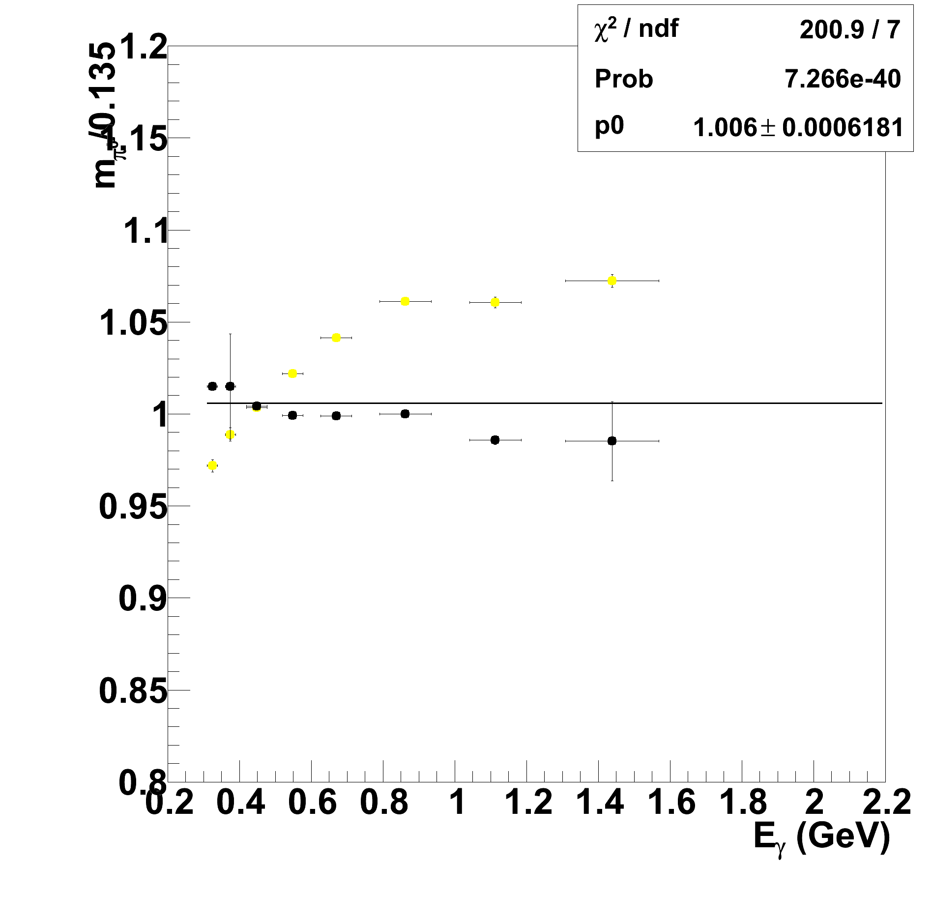
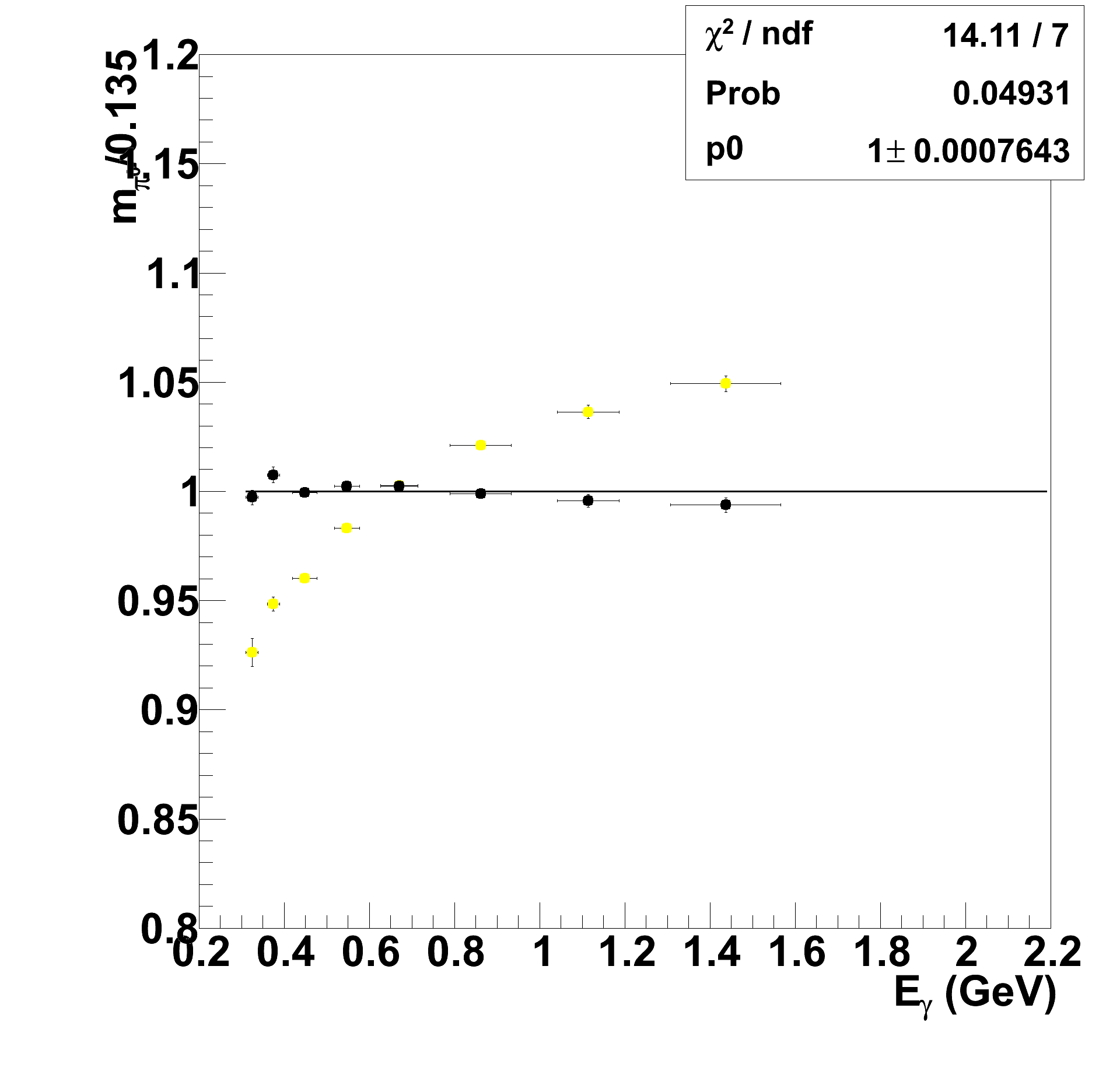
Plotted Pi0 invariant mass normalized to 0.135 GeV vs photon energy (E1, E2 in the same bin):
black for D/red for C points include photon energy correction, yellow - do not.
Black line corresponds to the linear fit of the corrected pi0 mass (with p0 in the box)

CARBON


LEAD


DEUTERIUM (from C)



R e s u l t.
Correction for Fe (+D):
1.116-0.09213/E+0.01007/(E*E)

IRON


DEUTERIUM (Iron)





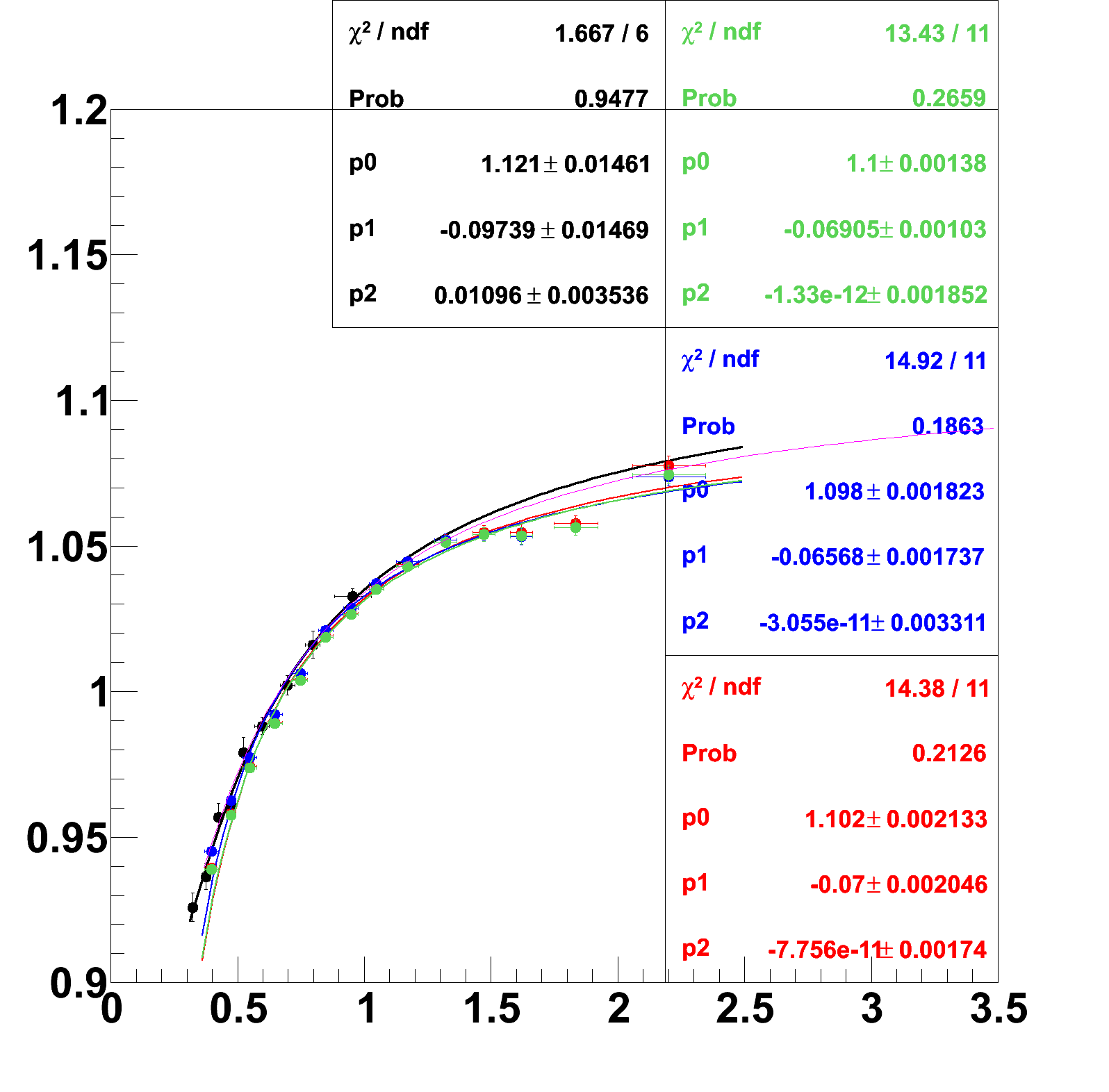
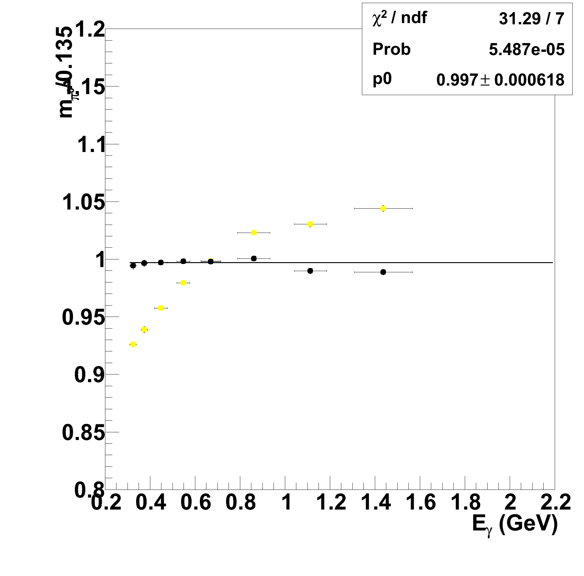
Fig.0a Pi0 invariant mass distribution for the D (black,top panel) and C (red,bottom).
Left plots have a z>0.4 cut imposed, whereas right plots are integrated over all kinematics.
Mean value of the invariant mass fit are given by parameter 'p4' in the box.
Before correction Pi0mass was +4.5% off its value, after -0.7% .


Procedure on the example of D+C.
Steps are described in Pass1 Step 1. Left is D. Right is C. Fig1


Step 2. Fig2


Fit. Fig.3


Sampling fraction. Fig.4



PASS1 Photon energy correction for each of three target sets.
Invariant mass of Pi0 was calculated from ECPB bank.


Carbon

Step 1
In Step1 the two photons such that |E1-E2|< 0.2*BinSize were selected. The correction factor was estimated : coor(E)= IM(Eg1,Eg2)/0.135, where
IM{Eg1,Eg2} = 2 x sqrt(Eg1 x Eg2 ) x sin(open_angle/2.)
Eg1 and Eg2 - photons' energies deposited in EC, open_angle = open_angle(X_ec,Y_ec,Z_ec).


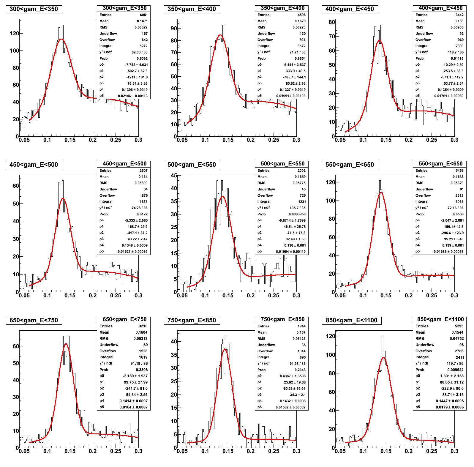
Fig.1 The data sample is divided into nine steps in energy, each fitted with Gaussian + (a + b x E + c x E^2)



Step 2
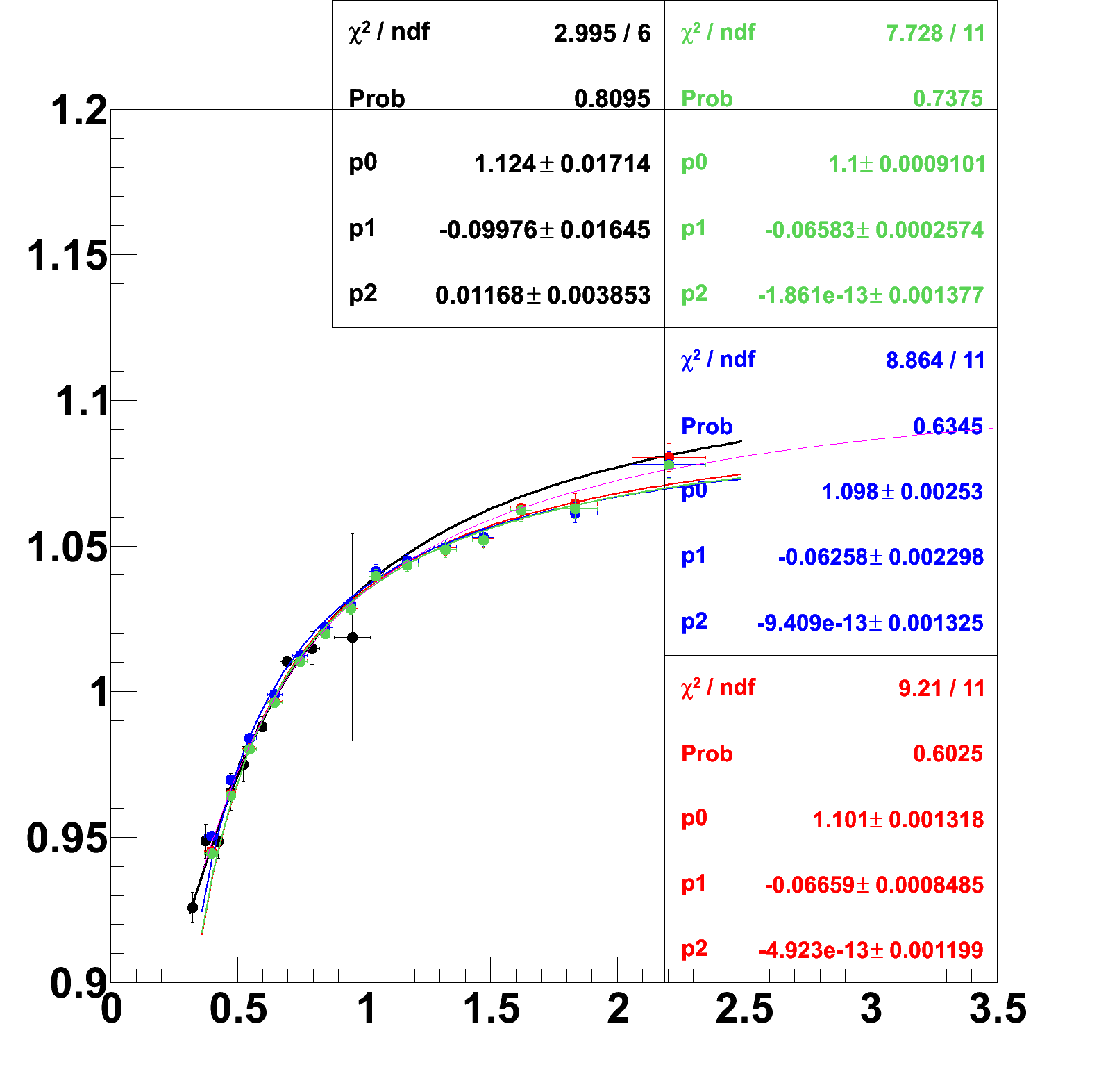
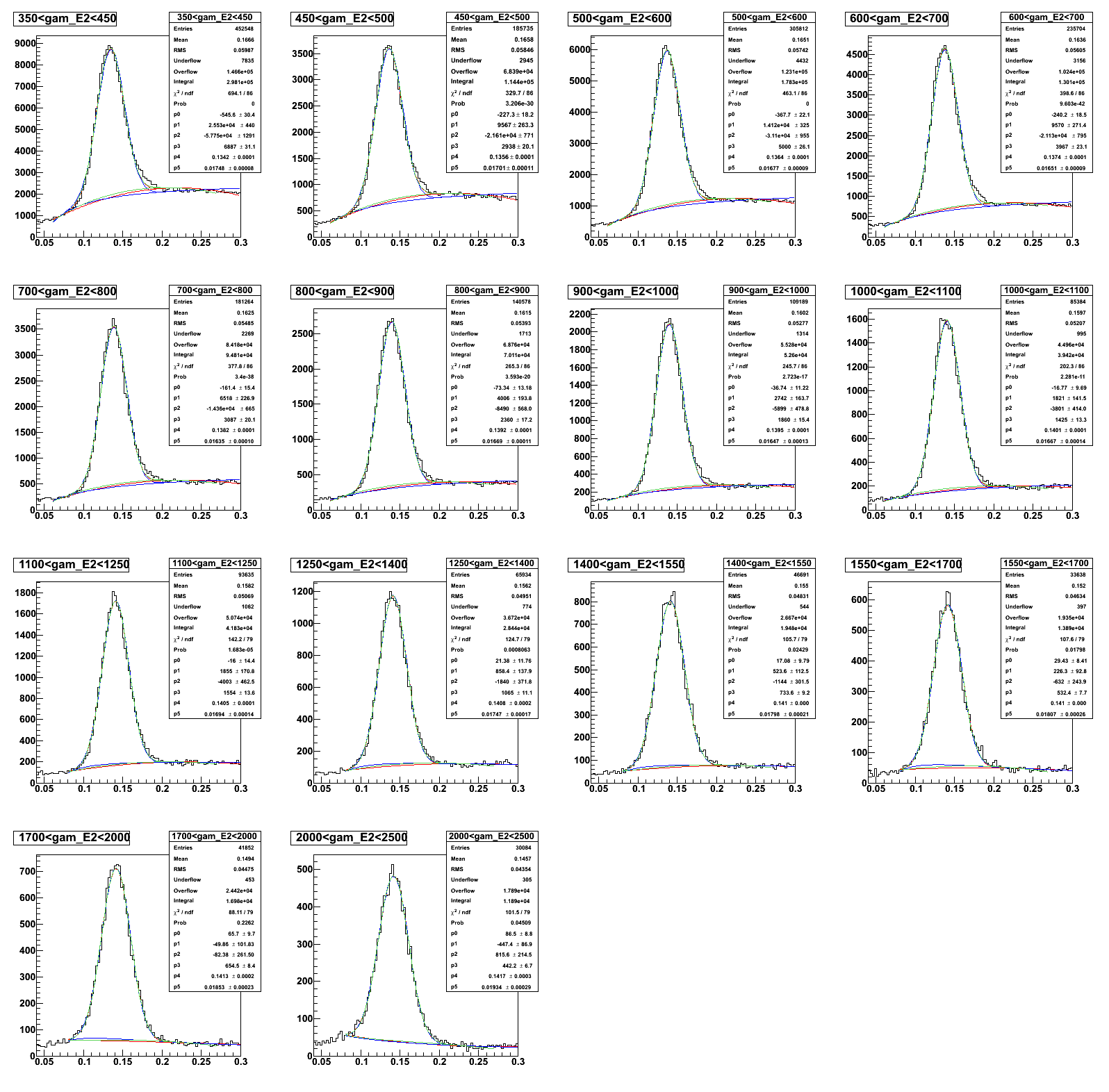
In Step2 E1(->E2 further corrected) or E2(->E1 further corrected) were limited to the range were the correction from Step1 is valid (0.3-1.0 GeV). The histograms were fitted using Gaus+Background. Three different colors correspond to various background functions:
a + b x E + c x E^2 (RED)
a + b/E + c/E^2 (BLUE)
a/E + b x E + c x E^2 (GREEN)
Fig.2



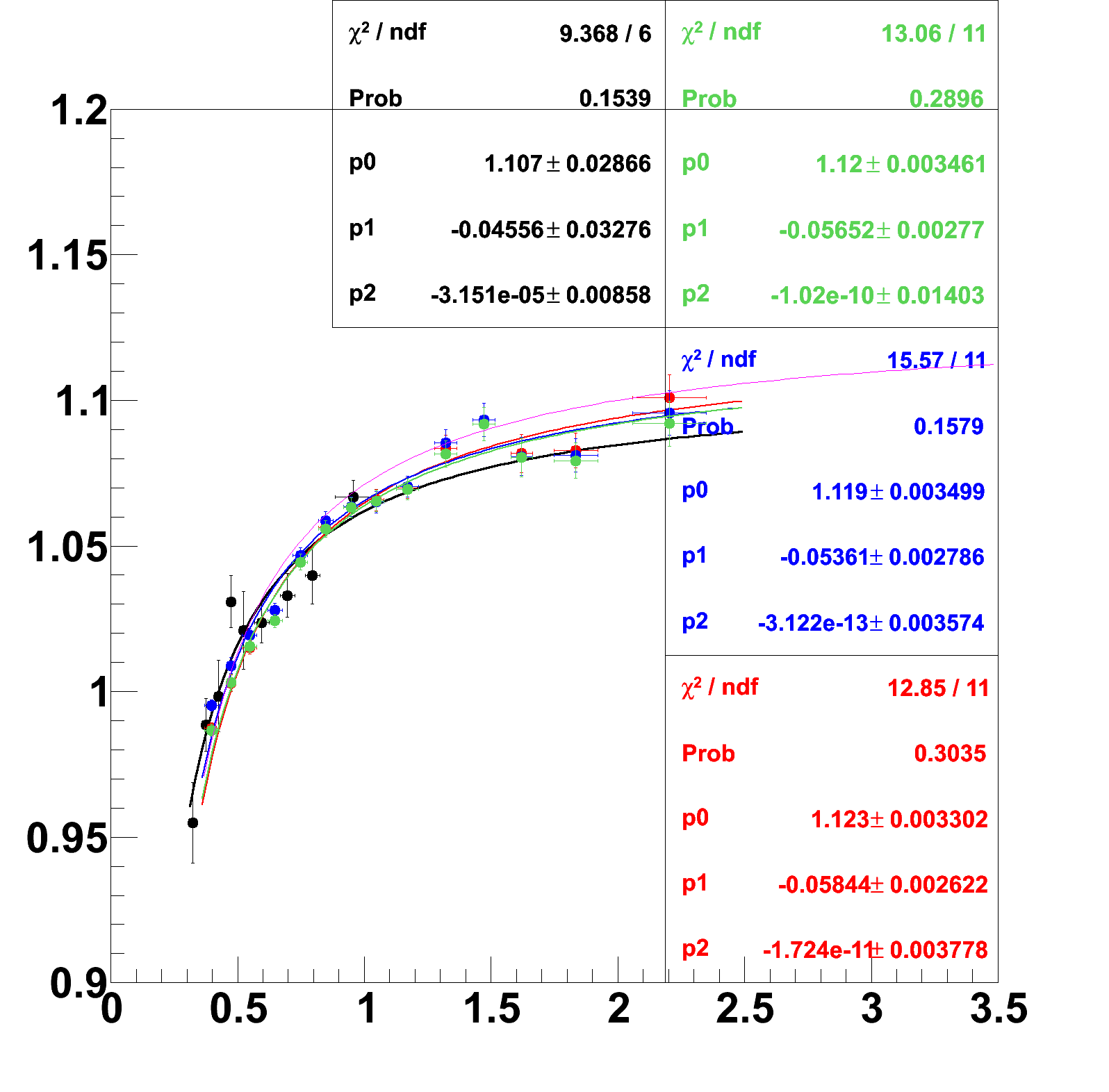
Fig.3 The mean value of the gaus / 0.135 is plotted versus E (where E = mean photon energy in bin, other photon in step1 range is corrected with previous parameters). Each set of points (red,blue, green) were fitted with earlier determined function: a + b/E + c/E^2. Parameters variations are small whithin errors, for several background shapes. For comparison, the points and fit obtained in step1 are drawn in black. On the right plot, a fit of the mean gaus/0.135 as a function of inverse energy:





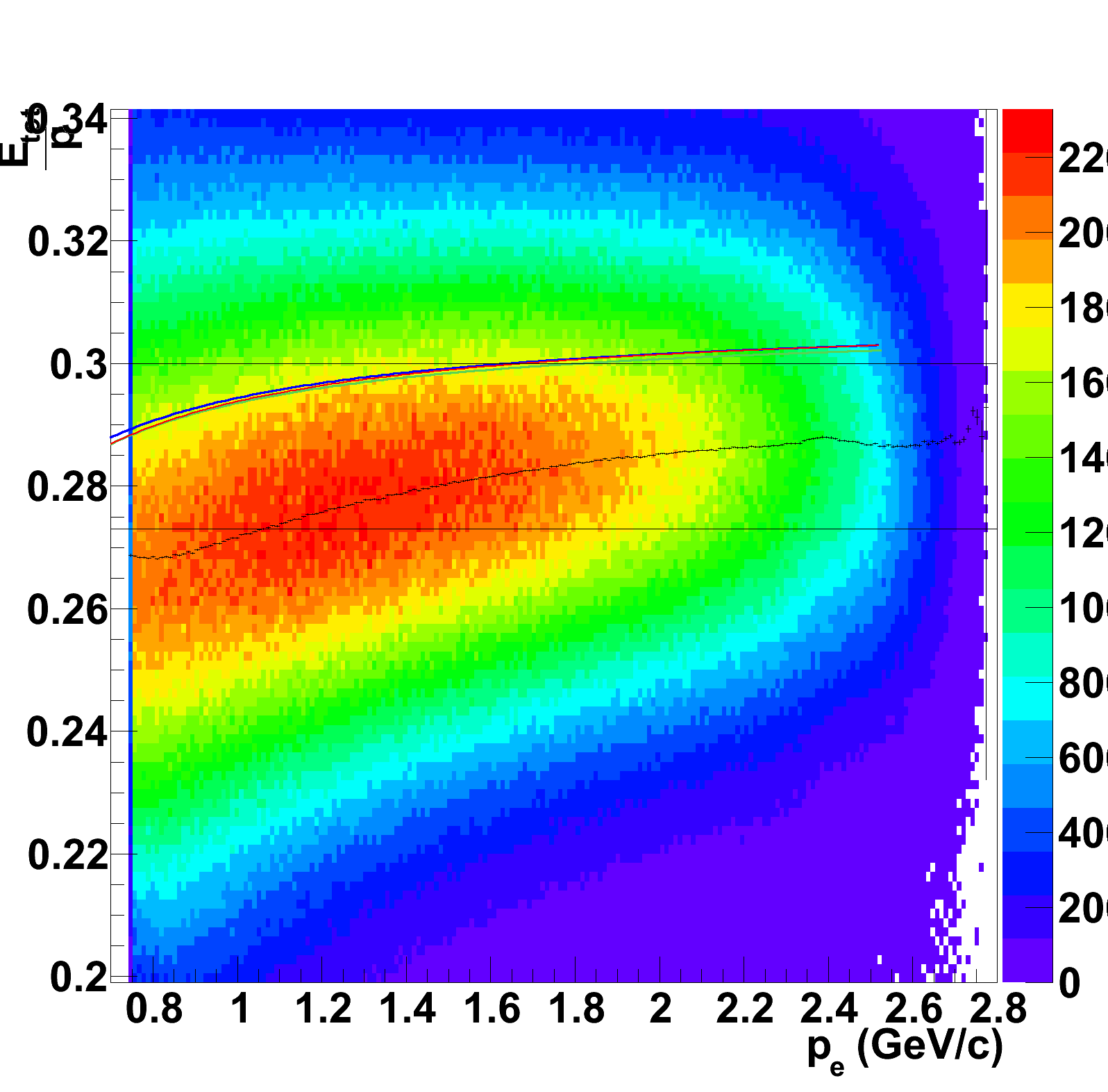
Fig.4 For comparison, the sampling fraction for electrons is illustrated below together with the photon's one corresponding to the corrections extracted with this method. The colored histogram is the electron sampling fraction, Etot/p vs p. Each slice in Y is fitted with a gaussian (ROOT method) resulting in the black scattered points for illustration of the approximate mean values (NB : the upper cut values comes from Hayk's analyzer, is too tight and can only shift the estimated means towards lower values). The 3 color curves are constructed by (0.273 x correction) as a function of corrected photon energy. The resulting discrepancy is less than 10%, but apparently opposite to what e1dvcs group has found



Step3

The last step is aimed to check the validity of photon energy correction determined earlier. Corrrection function corresponding to the 'red' background fit was chosen. Fig.5 Two photons with energies |Eg1-Eg2|<0.25*BinSize were choosen and corrected by the factor determined earlier:


Fig.6 The ratio of corrected mass value IM'( Eg1,/corr(Eg1), Eg2/corr(Eg2)) in each bin over pi0 mass is plotted. It is consistent with 1 within appr. 1.5%


Fig.7 Comparison of the Pi0 energies before and after correction. The slope on left plot is consistent with the behavior of the sampling fraction for the photon as a fuction of its momentum.


Fig.8. Carbon.Pi0 mass peak before and after correction. The photos energies are choosen above 0.35 MeV due to the rapid rase of the correction slope below this value.
Before correction: < Mass > = 0.137 MeV, Nevents = 431 682
After correction: < Mass > = 0.136 MeV, Nevents = 505 988




Deuterium Corresponding to Carbon target Step 1
Fig.1a



Step 2
Fig.2a



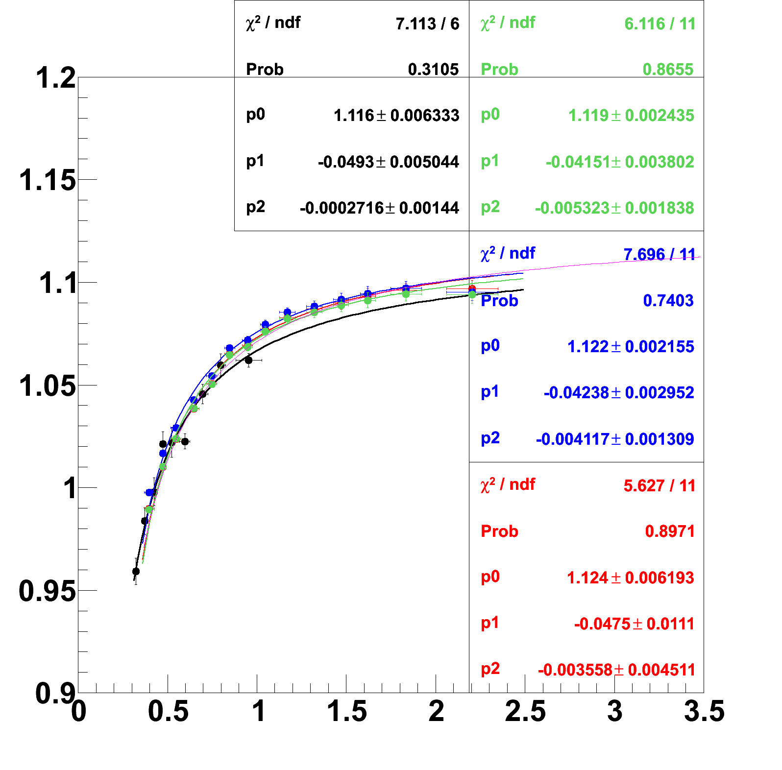
Fig.3a





Fig.4a



Step3

Fig.5a


Fig.6a:


Fig.8a. Pi0 mass peak before and after correction.
Before correction: < Mass > = 0.137 MeV, Nevents = 613 673
After correction: < Mass > = 0.1357 MeV,Nevents = 717 389




Determined correction is following: 1.099-0.04138/E - 0.00541/E*E



Iron+Deuterium Step 1
Fig.1 Left plot corresponds to Iron, right - to Deuterium



Step 2
Fig.2 Iron+Deut



Fig.3 Iron





Fig.3a Deut





Fig.4



Step3

Fig.5 Iron. Deut.




Fig.6:


Fig.8 Iron. Pi0 mass peak before and after correction.
Before correction: < Mass > = 0.132 MeV,Nevents = 396 547
After correction: < Mass > = 0.135 MeV,Nevents = 466 201


Fig.8a Deut. Pi0 mass peak before and after correction.
Before correction: = 0.132 MeV, Nevents = 730 927
After correction: = 0.135 MeV, Nevents = 853 788


Determined correction is following: 1.114-0.11/E + 0.0153/E*E



Lead+Deuterium Step 1
Fig.1 Left plot corresponds to Lead, right - to Deuterium



Step 2
Fig.2 Lead+Deut



Fig.3 Lead





Fig.3a Deut





Fig.4



Step3

Fig.5 Lead, Deut.




Fig.6:


Fig.8 Lead. Pi0 mass peak before and after correction.
Before correction: < Mass > = 0.1365 MeV, Nevents = 161 989
After correction: < Mass > = 0.135 MeV, Nevents = 191 230


Fig.8a Deut. Pi0 mass peak before and after correction.
Before correction: < Mass > = 0.136 MeV, Nevents = 846 777
After correction: < Mass > = 0.135 MeV, Nevents = 990 991


Determined correction is following: 1.099-0.04138/E - 0.00541/E*E (same as for Carbon)






------------------------------------------------------------------------------------------------------------------



Photon energy correction for two targets simulateneously.
Invariant mass of Pi0 was calculated from superposition of EVNT+ECPB banks

Step 1
In Step1 the two photons such that |E1-E2|<0.01 GeV were selected. The correction factor was estimated : coor(E)= IM(Eg1,Eg2)/0.135, where
IM{Eg1,Eg2} = 2 x sqrt(Eg1 x Eg2 ) x sin(open_angle/2.)
where Eg1, Eg2 - energy deposited/0.273 from ECPB bank, open_angle = open_angle(Px, Py,Pz) from EVNT bank.


Fig.1 The data sample is divided into nine steps in energy, each fitted with Gaussian + (a + b x E + c x E^2)



Fig.2 The mean values of pi0mass (gauss mean) plotted versus E (where E = mean pion energy in bin) were fitted using a Correction function of Step1 such that:
corr(E) = IM(Eg1,Eg2)/0.135 = 1.1 - 0.05/E +\- 0.0 (/E^2)



Step 2
In Step2 E1(->E2 further corrected) or E2(->E1 further corrected) were limited to the range were the correction from Step1 is valid (0.3-1.0 GeV). The histograms were fitted using Gaus+Background. Three different colors correspond to various background functions:
a + b x E + c x E^2 (RED)
a + b/E + c/E^2 (BLUE)
a/E + b x E + c x E^2 (GREEN)
Fig.3



Fig.4 The mean value of the gaus / 0.135 is plotted versus E (where E = mean photon energy in bin, other photon in step1 range is corrected with previous parameters). Each set of points (red,blue, green) were fitted with earlier determined function: a + b/E + c/E^2. Parameters variations are small whithin errors, for several background shapes. For comparison, the points and fit obtained in step1 are drawn in black. On the right plot, a fit of the mean gaus/0.135 as a function of inverse energy:




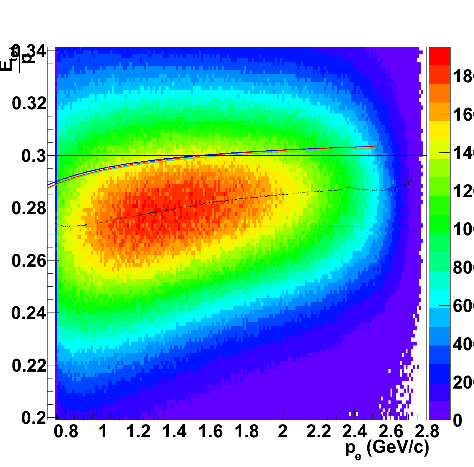
Fig.5 For comparison, the sampling fraction for electrons is illustrated below together with the photon's one corresponding to the corrections extracted with this method. The colored histogram is the electron sampling fraction, Etot/p vs p. Each slice in Y is fitted with a gaussian (ROOT method) resulting in the black scattered points for illustration of the approximate mean values (NB : the upper cut values comes from Hayk's analyzer, is too tight and can only shift the estimated means towards lower values). The 3 color curves are constructed by (0.273 x correction) as a function of corrected photon energy. The resulting discrepancy is less than 10%, but apparently opposite to what e1dvcs group has found



Step 3

The last step is aimed to check the validity of photon energy correction determined earlier. Corrrection function corresponding to the 'red' background fit was chosen. The ratio of corrected mass value IM'( Eg1,/corr(Eg1), Eg2/corr(Eg2)) over pi0 mass is consistent with 1 within appr. 1.5%
Fig.6 IM(Eg1/corr(Eg1),Eg2/corr(Eg2))/0.135 vs Pi0 Energy(GeV)


Fig.6a Mass before correction (black) and after (red)




Photon energy correction for each of two targets (deuterium and carbon)
Pi0Mass = 2*sqrt(Eg1)*sqrt(Eg2)*sin(theta/2),
where Eg = Edep/0.27 comes from ECPB bank and theta= theta(Px,Py,Pz) comes from EVNT bankx

Fig.7 Step1: left - deuterium, right - carbon


Fig.8 Step2


Fig.9
Deuterium correction factor: corr(E) = 1.115 - 0.0643/E + 0.004575/(E^2)
Carbon correction factor: corr(E) = 1.109 - 0.05066/E + 0.001643/(E^2)


Fig.10 Corrected mass corresponds to the red line for deuterium on the left and carbon on the right.




Additional plots
Fig.11 Opening angle (From ECPB) for 2 photon vs sum of their energy





Anaylsis made for Step 2
Fig.12 Check assymetric distributions of Eg1 and Eg2 in every bins





Fig.12a Eg1 is larger than Eg2, however due to correction first applied to the Eg1, its value shifts in some cases below Eg2




Fig.13 Gauss+Background fit start from the different values(violet=0.06, green=0.08, red=0.085) of invariant mass due to the EC reconstruction discrepancies at higher photon energies




Fig.13a