Level 2 trigger

**Table 1:** Level 2 and hit base events. Column 2- are all events with class type=3 (charged trigger),Column-3 and 4 are subsamples of Column 2 with event type=1 (LVLT2 accepted) and type=4 (LVLT2 rejected), Column-5 and 6 are tracks from HBTR without and with cut on class type=3, Column-7 all tracks with LVLT2 OK (including bit 1)
Run	evtclass=3	3/1	3/4	HBTR events	HBTR/3	LVL2 OK
20056	47700	47700		34251	31946	70000
20059	48561	31279	17282	26528	20737	48115
20077	51538	32335	19203	24831	19426	46594
20118	70000	46923	23077	31530	31530	46869

The comparison of Run 20056 and 20059, which were done under the same trigger conditions (bit 1 and 3 on), shows, that the number of hit base tracks for the same number of total events (70000) is increasing about 1.5 times (the ratio of corresponding numbers in column-6). Roughly 50% (excluding sector 4) of tracks passing through the Level 2, are giving an input in the hit base track bank (see Figs. 1,2). The difference in the number of tracks in events with identified tracks is shown in Fig. 3. The number of hit base tracks in different sectors for this two runs is similar and the ratio of hit based tracks to LVL2T tracks is exactly the same (see Fig.2). This probably means that the software and hardware rejection are performing in the same way. Comparison of hits from reconstructed tracks (RECSIS) with tracks identified by Level 2 hardware for different sectors is presented in Fig. 4. The main message of that plot, is, that almost 100% of reconstructed (RECSIS-HBTR) tracks have a correct sector identification on Level 2 hardware level. Very few tracks have 1 sector shifted between software and hardware. The tracks from HBTR bank rejected by the Level 2 versus the sector number are shown in Fig. 5. Majority of that rejected tracks have a sector properly identified by Level 2 hardware, and was rejected for some unknown reason. The number of rejected (miss-rejected) tracks is much lower when the neutral trigger (bit 1 ) is off, even if the tracks included in the consideration were all choosen to have event class(in HEAD bank) equal 3, which corresponds to the charged trigger. The kinematic distributions of rejected by Level 2 hit base tracks (less than 1% in worse case), are shown in the Fig. 6.

**Figure 1:** The number of LVL2 tracks (upper solid line in all plots) and corresponding number of hit based tracks from HBTR. The lower lines are solid Run 20059,dashed Run 20077 ,dotted Run 20118 and dash-dotted Run 20056.
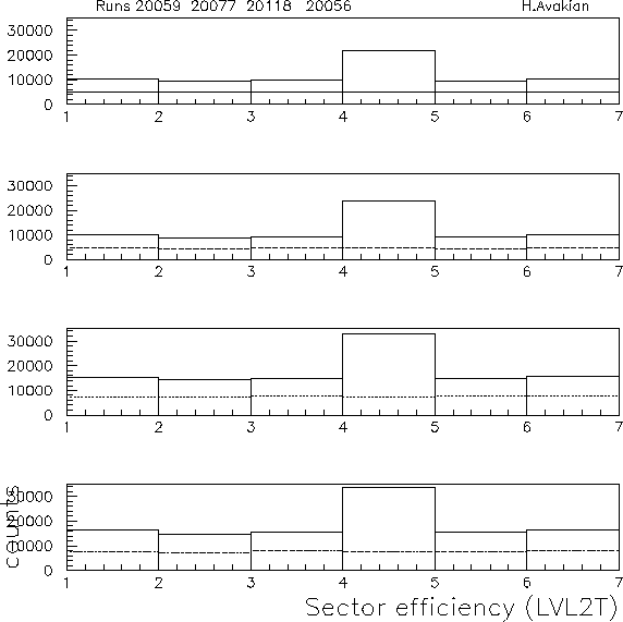$\begin{figure} \begin{center} \epsfig {file=sectornotrack.eps,width=14cm} \end{center} \end{figure}$

**Figure 2:** The ratio of hit based tracks from HBTR to the number of LVL2 tracks. (see. 1)
$\begin{figure} \begin{center} \epsfig {file=sectornotrackratio,width=14cm} \end{center} \end{figure}$

**Figure 3:** Difference in total number of tracks per event between Level 2 and hit base tracking.The bottom plot was done, without the sector 4 tracks. Sector 4 was malfunctioning during that runs.
$\begin{figure} \begin{center} \epsfig {file=lvlthits.eps,width=14cm} \end{center} \end{figure}$

**Figure 4:** LVL2 sector reconstruction efficiency. Shows the difference in the sector number, for tracks from HBTR (hit base tracking) and TGBI (Level 2 hardware). Zero means the sector is the same, and minus 1 means the sector is different (typically the neighboring one).
$\begin{figure} \begin{center} \epsfig {file=secineff.eps,width=14cm} \end{center} \end{figure}$

**Figure 5:** LVL2 sector inefficiency: Tracks in HBTR rejected by the Level 2 hardware. Rejected tracks mainly have hits in Level 2 appropriate sector information, but were marked as bad for some reason.
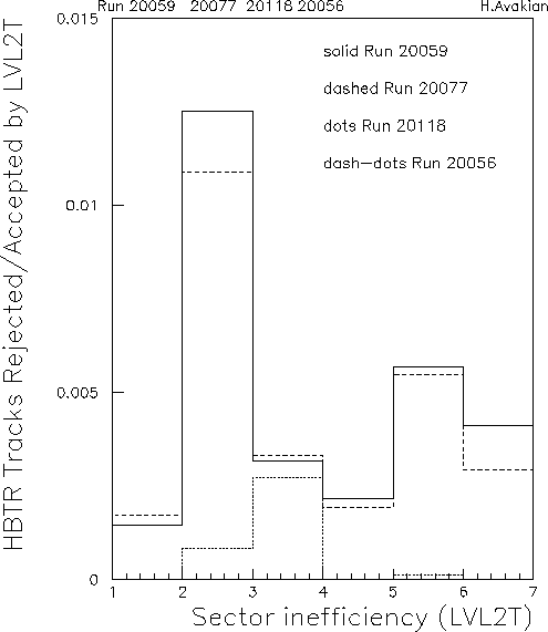$\begin{figure} \begin{center} \epsfig {file=sectoreff.eps,width=14cm} \end{center} \end{figure}$

**Figure 6:** Kinematic distributions of tracks from HBTR rejected by LVL2.
$\begin{figure} \begin{center} \epsfig {file=rejectdist.eps,width=14cm} \end{center} \end{figure}$